7. DTOcean Themes

7.1. Economics Module

The ‘economic assessment’ module takes the array configuration determined by the design modules (hydrodynamics, Electrical Sub-Systems, Moorings and Foundations, Installation, Operations and Maintenance) and estimates the LCOE for the project. The LCOE is the indicator used for benchmarking different possible solutions, and the global optimisation routine objective is to minimise it.

Within each design module there are economic functions that calculate the lifetime costs of the corresponding subsystem. These will be used as input for the LCOE calculation.

7.1.1. Architecture

The ‘economic assessment’ module is composed of a set of functions that are used to calculate the LCOE, which can be called separately or as a whole. The functions and their interactions with the inputs are presented in a diagrammatic form in Fig. 7.1.

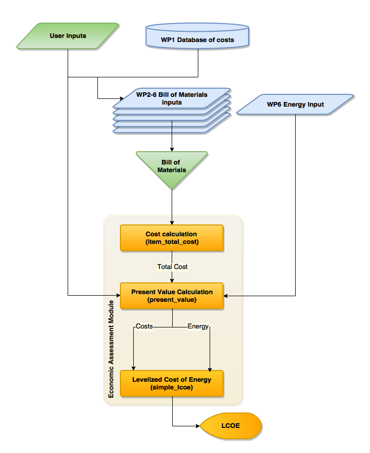
Fig. 7.1 Flowchart of Economic Assessment Module

7.1.2. Functional specifications

7.1.2.1. Inputs

The Economics module requires inputs from other modules and from the user. Note that the inputs from other modules can always be overwritten by the user.

The Bill of Materials is generated by the core from the outputs of the other design modules. It is formatted as a pandas tables, with the following fields:

• item: identifier column, not used in the function
• quantity: number of units of item
• unitary_cost: cost per unit of the item. It assumes that it matches the units of the quantity
• project_year: year relative to the start of the project when the cost occurs (from year 0 to the end of the project)

The second set of inputs generated by the tool relates to the energy production. It also formatted as a pandas table, with the following columns

• project_year: year relative to the start of the project when the cost occurs (from year 0 to the end of the project)
• energy: final annual energy output. This value accounts for the hydrodynamic interaction, transmission losses and downtime losses

The project_capacity input, referring to project capacity in MW, is an output from the Array Hydrodynamic module, by using the number of devices output and the user input on device rating.

The inputs a_energy_wo_elosses and a_energy_wo_availability are outputs from the the Array hydrodynamic and Electrical sub-systems modules, respectively. The input a_energy_wo_elosses indicates the average annual unconstrained energy production, before electrical losses; while a_energy_wo_availability indicates the average annual energy production accounting for electrical losses, but without accounting for availability.

From the user, the following inputs are required:

• project_lifetime: duration of the project in number of years
• discount_rate: discount rate for the project in analysis. The discount rate is dependent on the investor’s valuation of risk and other investment opportunities.

7.1.2.2. Outputs

The main output of the economics theme module is the levelized cost of energy (LCOE) of the project, expressed in €/MW. The building blocks of the LCOE calculation, CAPEX, OPEX and Annual Energy Production, are also outputs of the module

This allows for the representation of the contribution of CAPEX and OPEX to the LCOE, or the contribution of each sub-system/module.

7.2. Reliability Assessment Module

Reliability assessment module aims at assessing the reliability of the array configuration determined by the design modules (Electrical Sub-Systems and Moorings and Foundations). RAM conducts reliability calculations for i) the user and ii) to inform operations and maintenance requirements of the O&M module.

The purpose of the RAM is then to:

• Generate a system-level reliability equation based on the inter-relationships between sub-systems and components (as specified by the Electrical Sub-Systems and Moorings and Foundations component hierarchies and by the user)
• Provide the user with the opportunity to populate sub-systems not covered by the DTOcean software (e.g. power take-off, control system) using a GUI-based Reliability Block Diagram
• Consider multiple failure severity classes (i.e. critical and non-critical) to inform repair action maintenance scheduling. This will represent a simplified approach to Failure Mode and Effects Analysis (FMEA)
• Carry out normal, optimistic an d pessimistic reliability calculations to determine estimation sensitivity to failure rate variability and quality analysis
• Provide the time-dependent failure estimation model (in the O&M module) with the Time to failure (TTF) of components within the system

RAM produces:

• A pass/fail Boolean compared to user-defined threshold
• Distribution of system reliability (%) from mission start to mission end (0≤t≤T).
• Mean time to failure (MTTF) of the system, sub-systems and components presented to the user in a tree format
• Risk Priority Numbers (RPNs)

7.2.1. Architecture

The RAM comprises two Python modules (figure below). RAM_Main.py acts as an interface between the user and the module and also calls the functions within the RAM. RAM_Core.py comprises the classes and functions required to carry out statistical analysis of the system. As can be seen from the interactions diagram with RAM_Core.py there is interaction between the functions within the Syshier class.

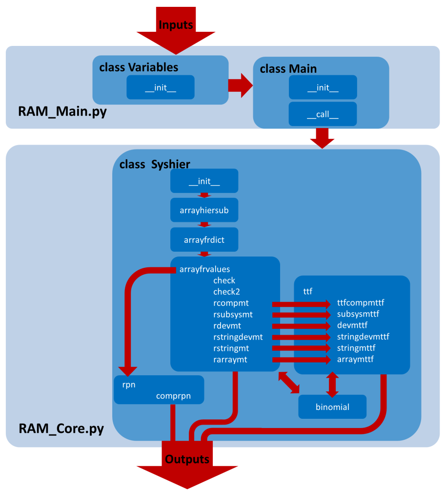
Fig. 7.2 Interaction between the various classes and methods of the Reliability Assessment sub-module

7.2.2. Functional specifications

7.2.2.1. Inputs

Inputs to the Reliability assessment module are provided by the electrical module, the moorings and foundations module, the database and the user. A list of the inputs required are as follows:

Fig. 7.3 Inputs to the Reliability assessment module

7.3. Environmental Impact Assessment module (EIAM)

7.3.1. Introduction

The purpose of the Environmental Impact Assessment Module (EIAM) is to assess the environmental impacts generated by the various technological choices to optimize an array of wave or tidal devices. This is done by a set of specific functions (e.g. collision risk, noise…) that are able to qualify and quantify the potential pressures generated by the array of wave or tidal devices on the marine environment. The EIAM provides a rating (overall score and detailed by modules) for various technological choices selected in the tools.

The approach used here is based on the concept of environmental effects generated by ‘stressors’ and the related sensibility of ‘receptors’ to these effects. A stressor is any physical, chemical, or biological entity that can induce an adverse response. Stressors may adversely affect specific physical resources of marine ecosystems that interact directly with the biological components of these ecosystems: including plants and animals.

Within the above framework, it is therefore a matter to systematically identify and evaluate the relationships between all stressors and their impact on receptors. In order to achieve this, a set of environmental functions are considered to determine environmental scores (through specific mathematical functions). 13 functions have been defined, 10 related to negative impacts and 3 related to positive impacts (Reef effect, Reserve effect and resting place effect). The list of the different issues taken into account in the EIAM is given in the Fig. 7.4.

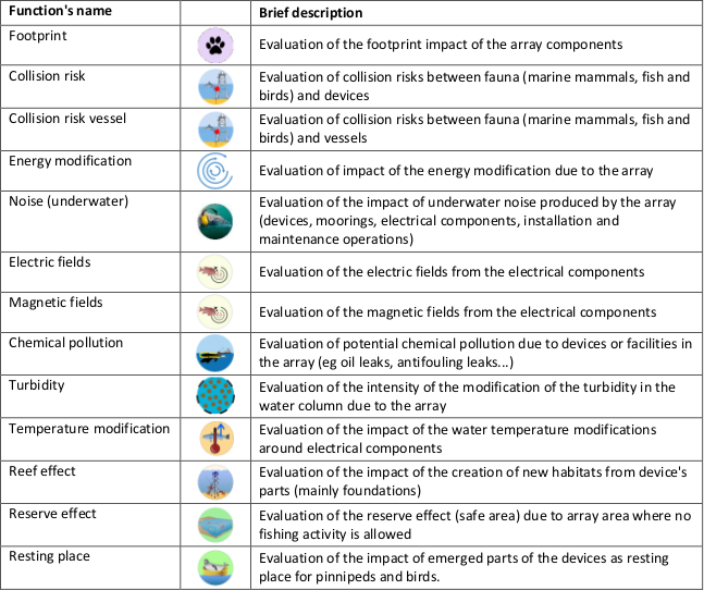
Fig. 7.4 List of environmental impacts assessed by DTOcean

Each function is specifically allocated to the different DTOcean modules (Hydrodynamics, Electrical Sub-Systems, Mooring and Foundations…), as each module involves different stressors depending on its purpose. Fig. 7.5 shows which functions are assessed for each of the DTOcean modules. Behind these allocations issues / module lie specific related mathematical functions. The description of these functions is available in the technical user manual.

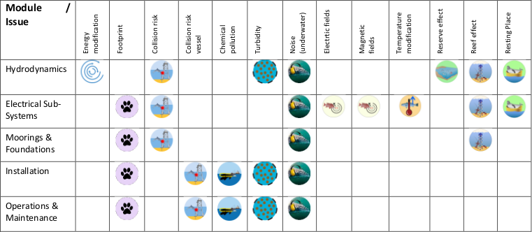
Fig. 7.5 Environmental issues associated with each DTOcean modules

7.3.2. Architecture

The architecture is based on a scoring system using mathematical functions to assess the environmental impacts. The process of these functions produces numerical values (from function’s scores) that are converted to Environment Impact Score (EIS) ranging from +50 to -100 (scale shown in Fig. 7.6). The mathematical detail of each function is available in the technical manual.

Fig. 7.6 Environmental Impact Score (EIS) scale

The scoring allocation system is generic for each environmental function and is based on three main steps, summarized in Fig. 7.7 and in the description below:

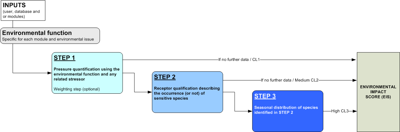
Fig. 7.7 Scoring architecture for the Environmental Impact Assessment Module (EIAM)

where CL = Level of Confidence: 1 Low, 2 Medium and 3 High.

• STEP 1: quantification of the ‘pressure’ generated by the stressors

The quantification of the pressure is obtained from the run of the selected environmental functions which produced the Pressure Score (PS). The PS ranges from 0 to 5 for the all functions where 5 corresponds to the highest effect, negative or positive, depending on the function. The PS is then adjusted to a new numerical value called the Pressure Score adjusted (PSa) through a ‘weighting protocol’ by multiplying the PS with a coefficient ranging from 0 to 1. This happens if local environmental factors exist, which are independent from the receptors, and are not included in the function’s formula. If no weighting is generated, a default value of 1 is used, with the precautionary principle prevalent throughout the EIAM process. At this stage the level of confidence is at its lowest.

• STEP 2: quantification of the receptor sensitivity

The second step is triggered if the user is able to indicate the existence of receptors onsite. Step 2 uses the score initially generated in step 1 and then adjusts it depending on the receptor’s sensitivity by multiplying the PSa with the Receptor Sensitivity coefficient (RS), which ranges from 0 to 5, unless the user has no receptor data, in which case the RS is assumed to be 5. This process leads to the Receptor Sensitivity Score (RSS). The different receptors are gathered within main classes reflecting their sensitivity to pressure. The user will have to choose between these different main classes of receptors that will be characterized by having RS values ranging from 0 to 5 for low to high sensitivity, respectively. When several receptors are identified onsite, the most sensitive receptors will be considered for the EIS calculations. To ultimately obtain the EIS a linear mapping is applied and specific calibration tables are used to convert RSS to EIS. In the case where the user declares a receptor that is regulatory protected (list provided by the database), by default this will automatically lead to an EIS of -100. If the user is able to provide details about the existence of receptors, the level of confidence increases to medium.

• STEP 3: qualification of the seasonal distribution of receptors

The last step is triggered if the user has monthly data for the existence of receptors onsite. The step then modulates the final EIS to take into account less sensitive receptors when the highest sensitive receptors are declared absent. Step 3 is similar to step 2 for each specific receptor declared onsite and the EIS is equal to 0 for any receptors absent in a particular month. For each month, the EIS is given by most sensitive species present. If monthly data are lacking the tool will consider the receptor is present throughout the year.

If the user has such monthly data, the level of confidence is at its highest. Functional Specifications

7.3.2.1. Inputs

The EIAM requires some inputs to be able to provide an EIS. These inputs are provided by the user and the other DTOcean modules and are listed in the table below, grouped by module.

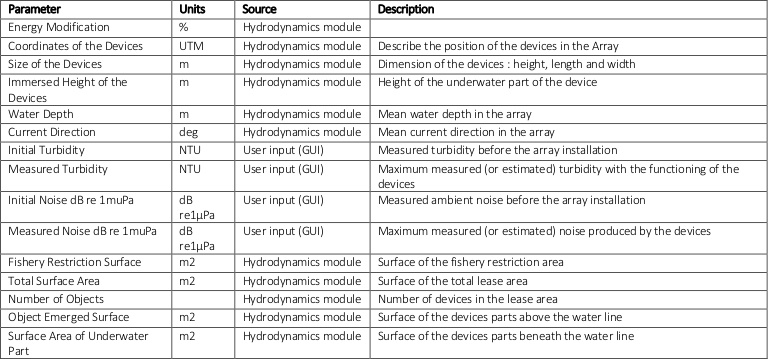
Fig. 7.8 EIAM inputs related to hydrodynamics (Name, unit, source and description)

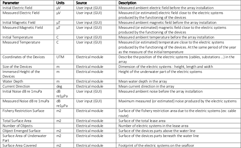
Fig. 7.9 EIAM inputs related to electrical architecture (Name, unit, source and description)

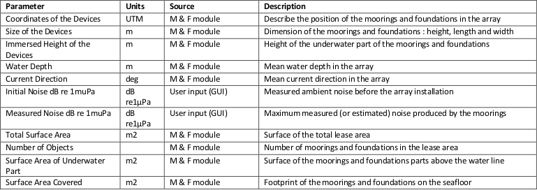
Fig. 7.10 EIAM inputs related to moorings and foundations (Name, unit, source and description)

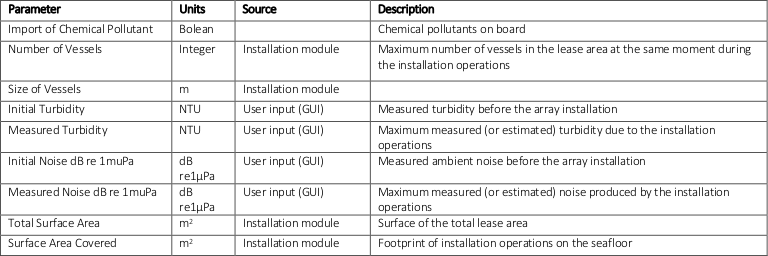
Fig. 7.11 EIAM inputs related to installation (Name, unit, source and description)

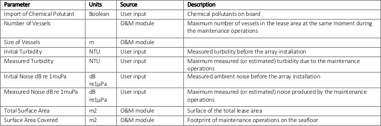
Fig. 7.12 EIAM inputs related to operations and maintenance (Name, unit, source and description)

Regarding noise measurement unit, the EIAM (for the pressure functions and the receptor sensitivity) uses dB re1µPa as main unit. The user has to make sure about using this unit. Indeed in some MRE projects impact assessments, the common noise measurement unit produced by the background of devices is ‘dB re 1µPa²’. The Fig. 7.13 shows that these two units are different.

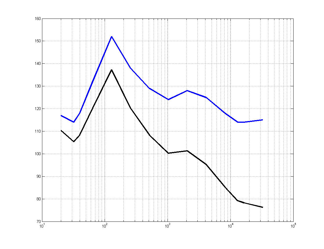
Fig. 7.13 Example of the noise radiated by an operating tidal current turbine. (In blue the Third Octave Band SPL [dB re 1µPa] (could have been Wide Band SPL = one value) and in black, the Power Spectrum Density Level [dB re 1µPa²/Hz])

To achieve the STEP 1, the Pressure score is adjusted through a weighting protocol in order to better characterise the environmental impact. In that context, weighting protocol are associated to some modules and related functions. 11 weighting parameters categories have been defined and are described in Fig. 7.14.

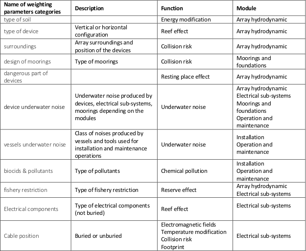
Fig. 7.14 Weighting parameters categories descriptions with functions and modules assigned

Details about values assigned to each weighting parameters categories are given in the following tables:

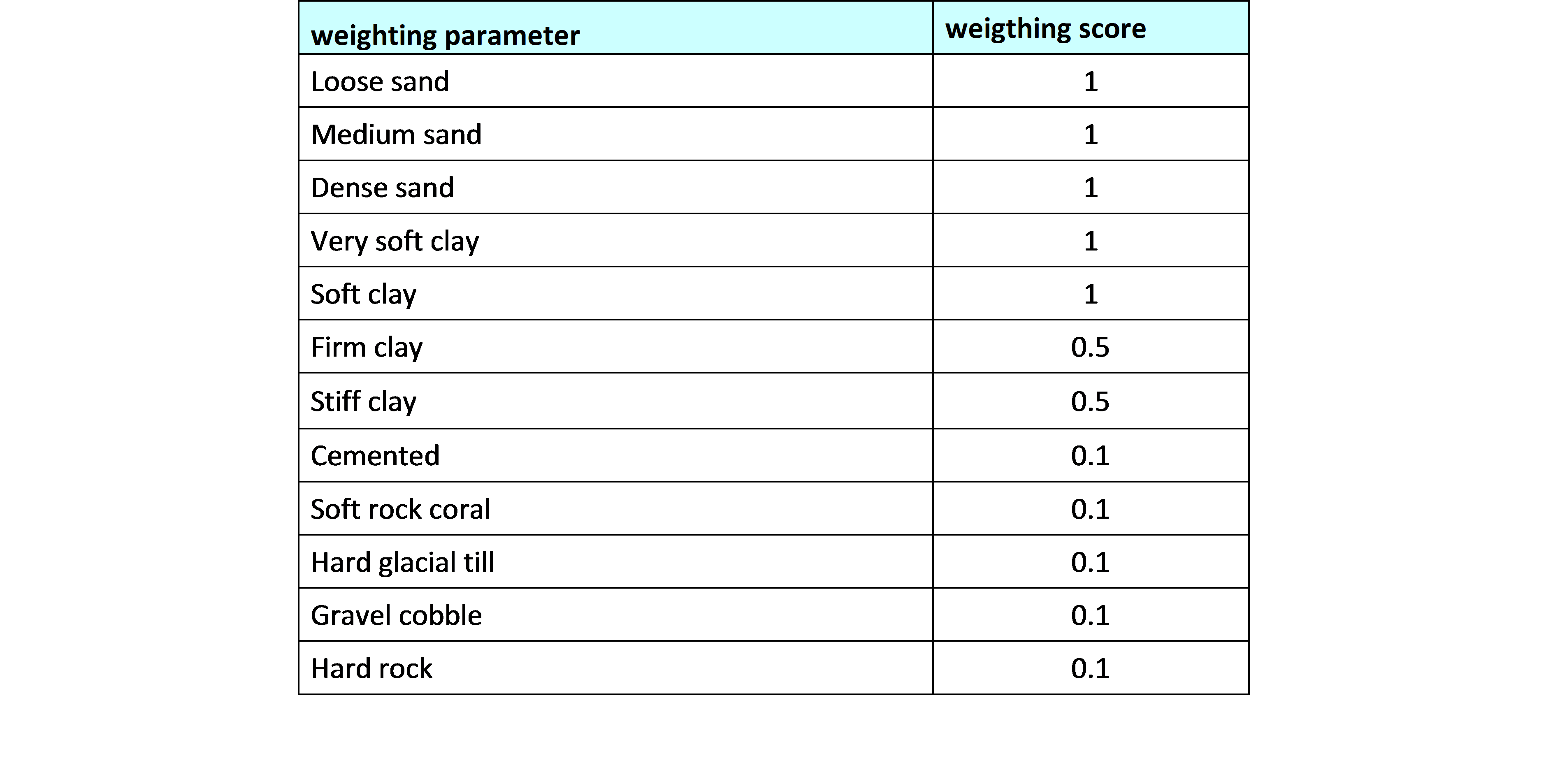
Fig. 7.15 Weighting parameters and scores associated for soil

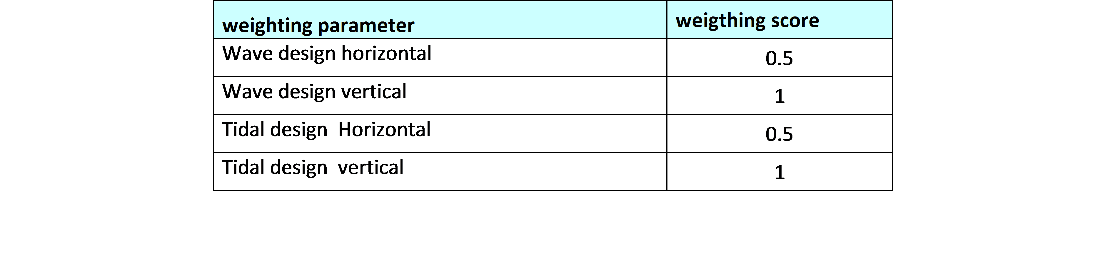
Fig. 7.16 Weighting parameters and scores associated to technologies

Fig. 7.17 Weighting parameters and scores associated to surroundings

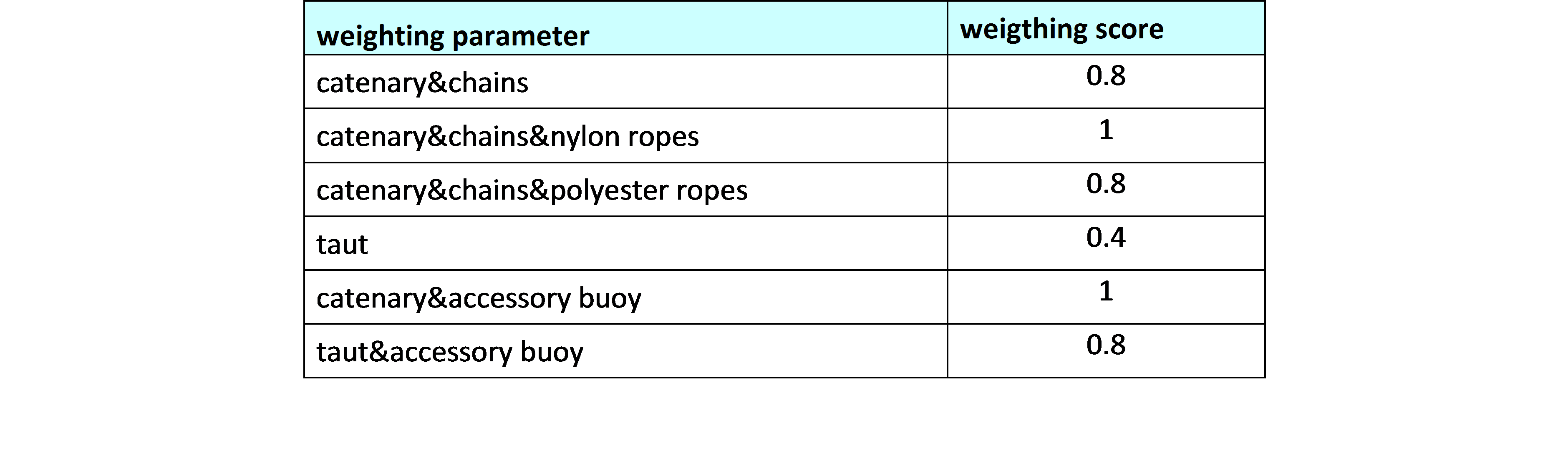
Fig. 7.18 Weighting parameters and scores associated to Moorings

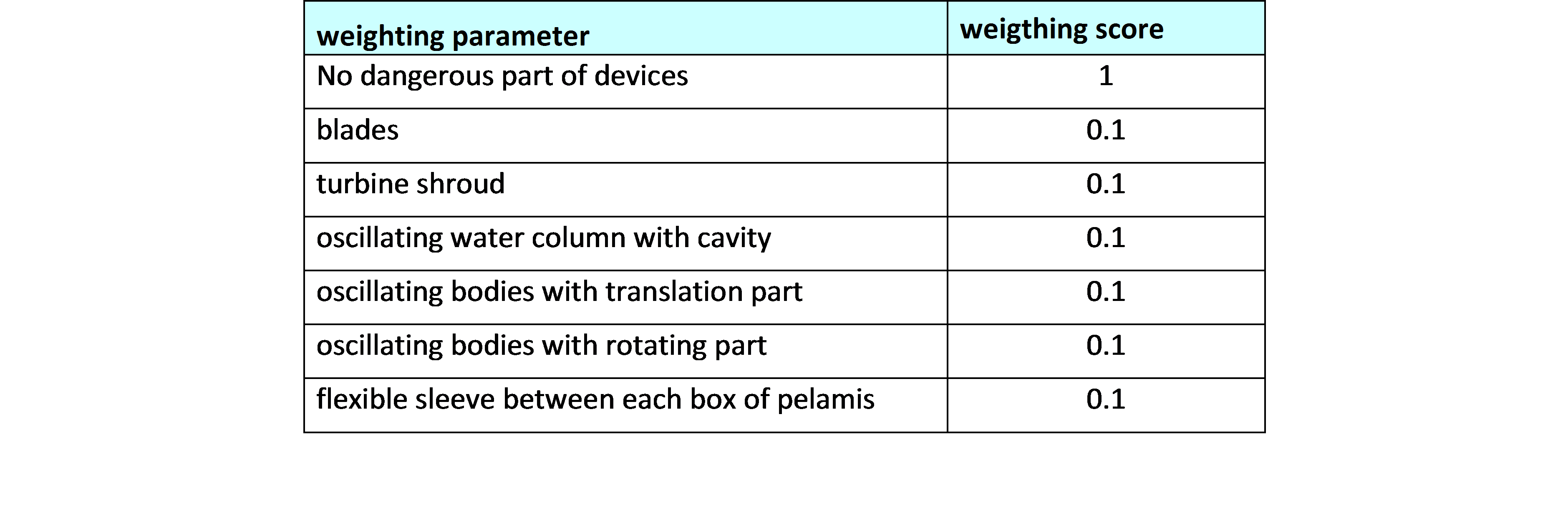
Fig. 7.19 Weighting parameters and scores associated to Dangerous parts of devices

Fig. 7.20 Weighting parameters and scores associated to Device underwater noise (device, electrical components, moorings)

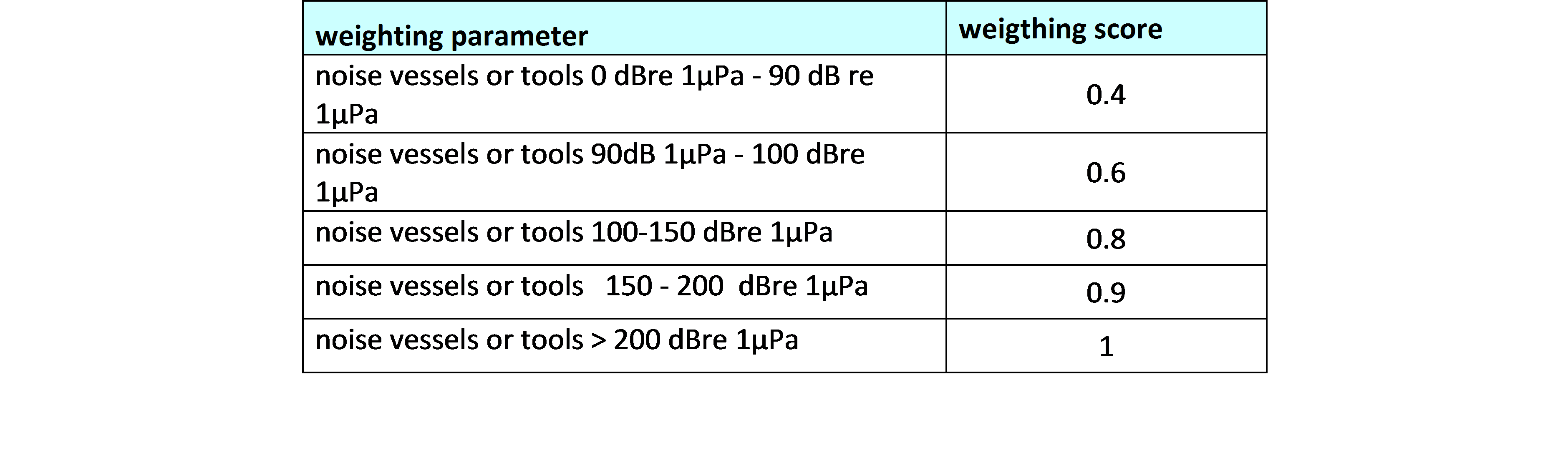
Fig. 7.21 Weighting parameters and scores associated to Vessel underwater noise

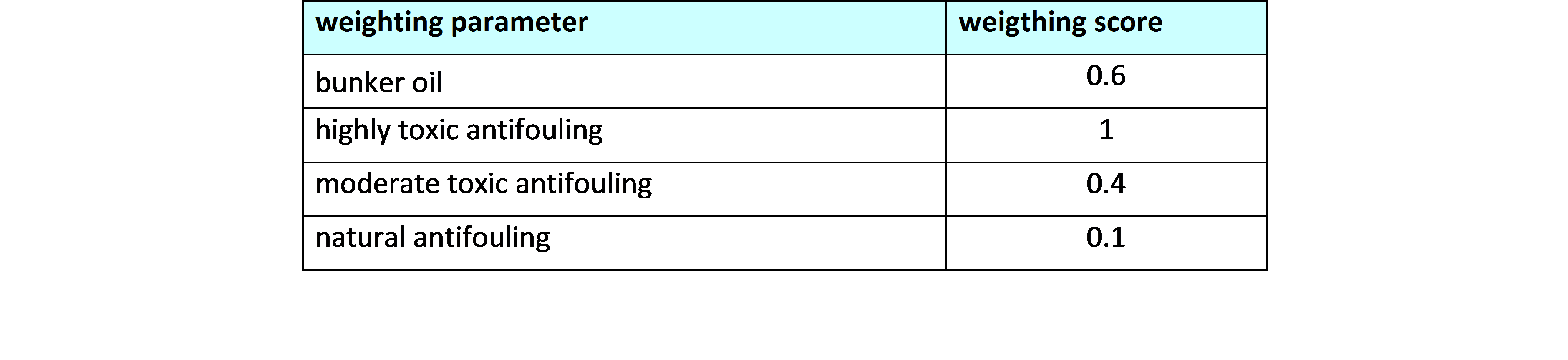
Fig. 7.22 Weighting parameters and scores associated to Biocids and pollutants

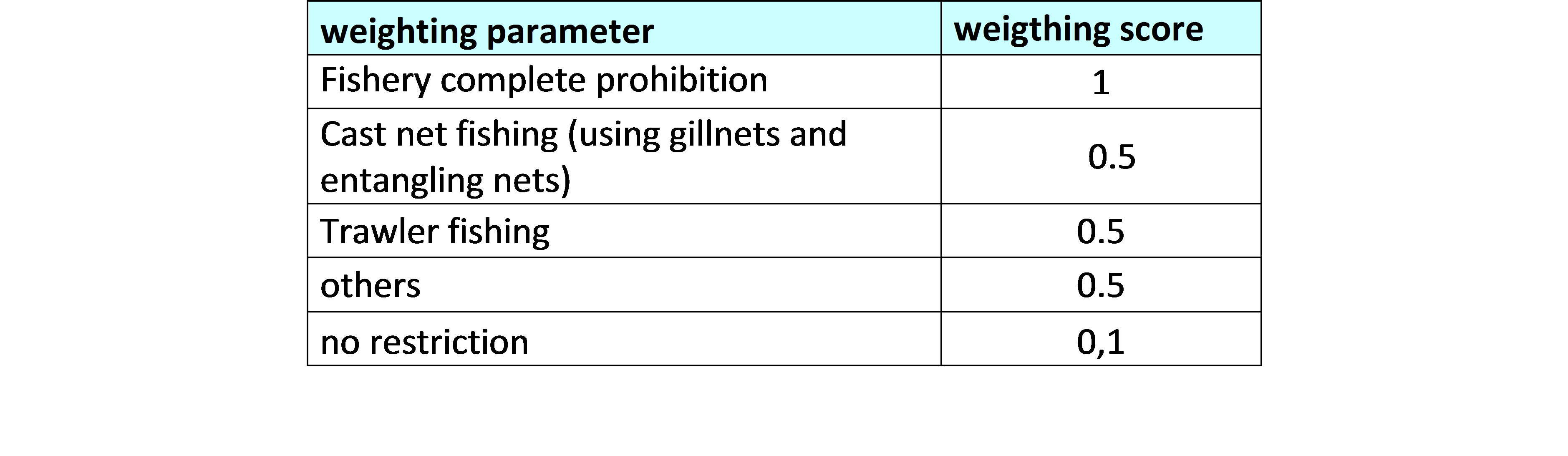
Fig. 7.23 Weighting parameters and scores associated to Fishery restriction

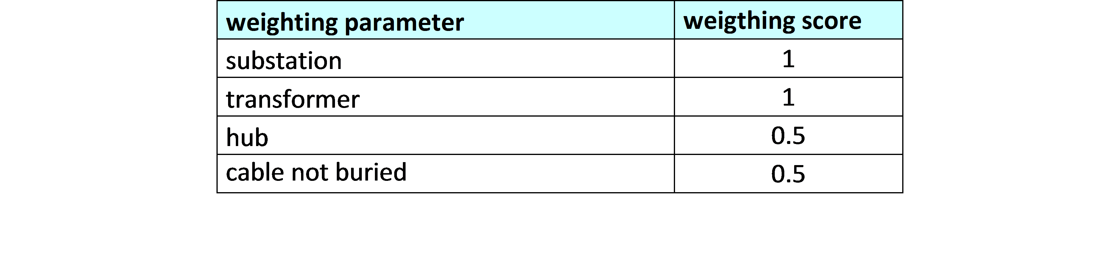
Fig. 7.24 Weighting parameters and scores associated to Extern electrical components

Fig. 7.25 Cable position category: Weighting parameters and scores associated

To qualify the receptor sensitivity (STEP 2), the user could be asked to better define the receptor present in the area. The main receptor categories are given in Fig. 7.26. A list of 13 receptor categories has been defined for the all EIAM.

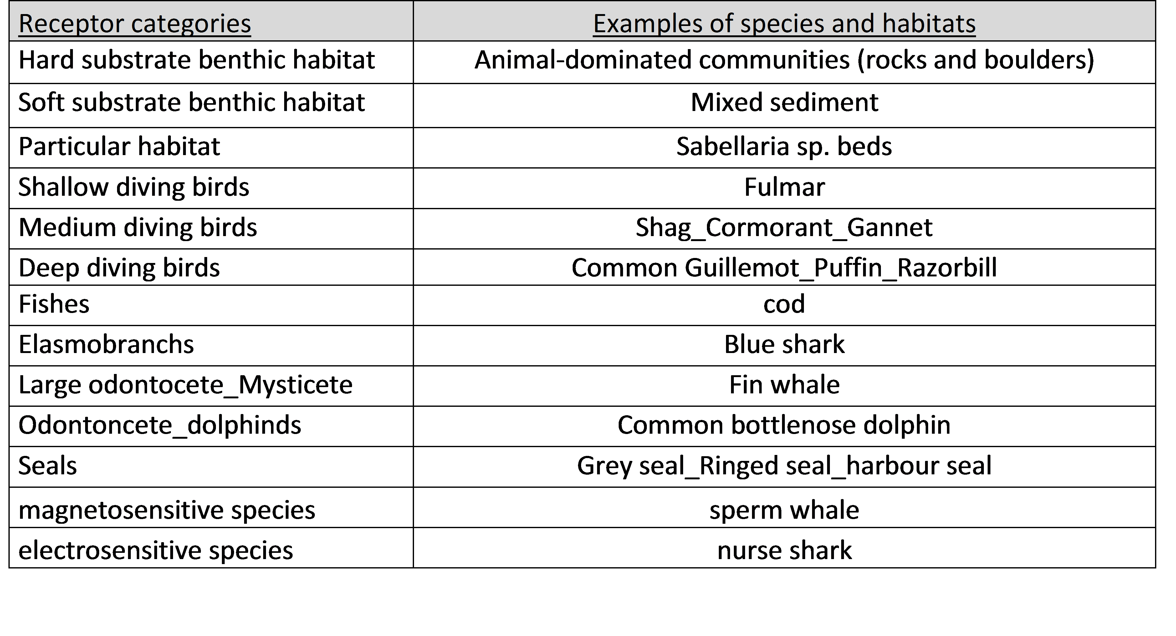
Fig. 7.26 Receptor categories

For each function in each module, a specific score is assigned to each relevant receptor categories depending on the sensitivity of each category to the pressure.

The Fig. 7.27 shows the example of the scores assigned to the receptor categories for the collision risk function in the hydrodynamics module.

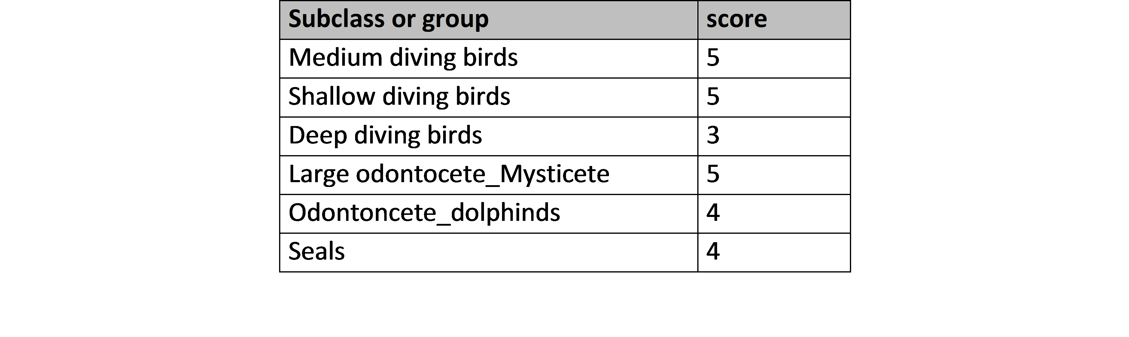
Fig. 7.27 Receptor sensitivity scores example for the collision risk function in the hydrodynamics module

As most marine mammals, birds and reptiles are protected by European regulations (Bonn convention, Berne convention, Birds directive, Ascobans, Accobam…), a “red list” has been established in the EIAM for those with the highest level of protection. The user has the possibility to indicate the occurrence of one (or more) of these protected species on top of the main receptor categories.

The list is presented in Fig. 7.28. The 26 species are baleen whales species classified by the annex I of the Bonn Convention. The bird species in the list are also classified by the annex I of the birds directive and the reptiles species by the annex IV of the Habitats directive.

Reminder: If the user declares the presence of a receptor that is highly protected in the European regulations so included within the “red list” (list provided internally in the tool), by default this choice will automatically lead to an EIS of -100.

Fig. 7.28 “Red list” constituted by highly protected species in the European regulations

Finally in order to proceed STEP 3, inputs requested are related to the seasonal distribution of receptors. The last step of the EIAM process takes into account the seasonal distribution of receptors onsite to modulate the receptor sensitivity. For each environmental function the EIAM proposed to the user the possibility to define the monthly distribution of the ‘selected’ receptors. The Fig. 7.29 presents an example of the required inputs for the 6 receptors relevant to the collision risk function of the electrical sub-systems module.

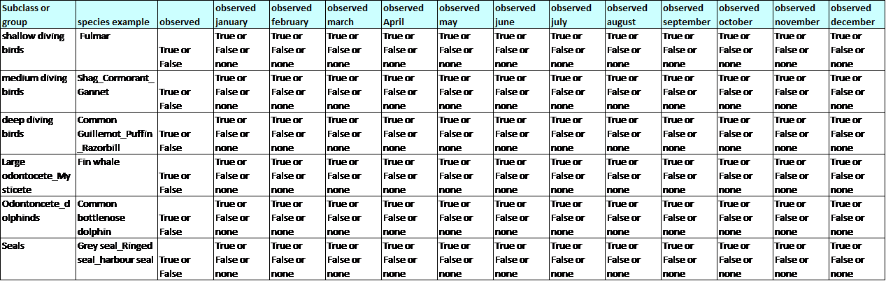
Fig. 7.29 Example of receptor seasonal distribution inputs for the collision risk function of the electrical sub-systems module

7.3.2.2. Execution

This part of the manual explains how the EIAM with the three steps presented below is executed within the GUI.

• STEP 1 : Quantification of the ‘pressure’ generated by the stressors
  • General inputs

When inputs are provided by the other modules of the tool, there is no special step to proceed in the GUI for the execution of EIAM.

Fig. 7.30 Example of the GUI (EIAM pipeline) as lease boundary for input directly provided by the hydrodynamics module

For inputs provided by the user, these inputs have to be entered manually through a widget within the GUI as shown in Fig. 7.31.

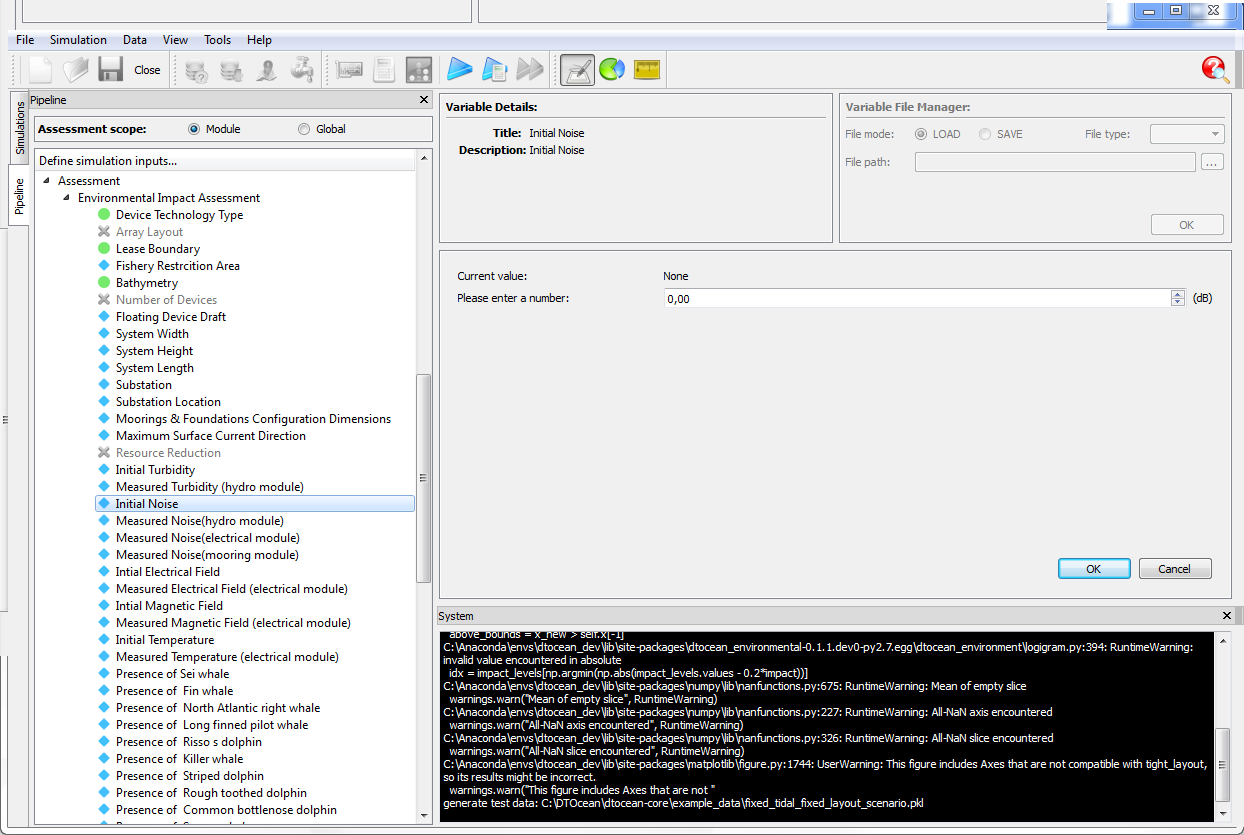
Fig. 7.31 Example of input to be provided by the user directly by the GUI

• Weighting protocol

For each weighting parameter, related to the relevant functions and modules, a dropdown menu allows the user to select the value in preselected lists. An example is presented below.

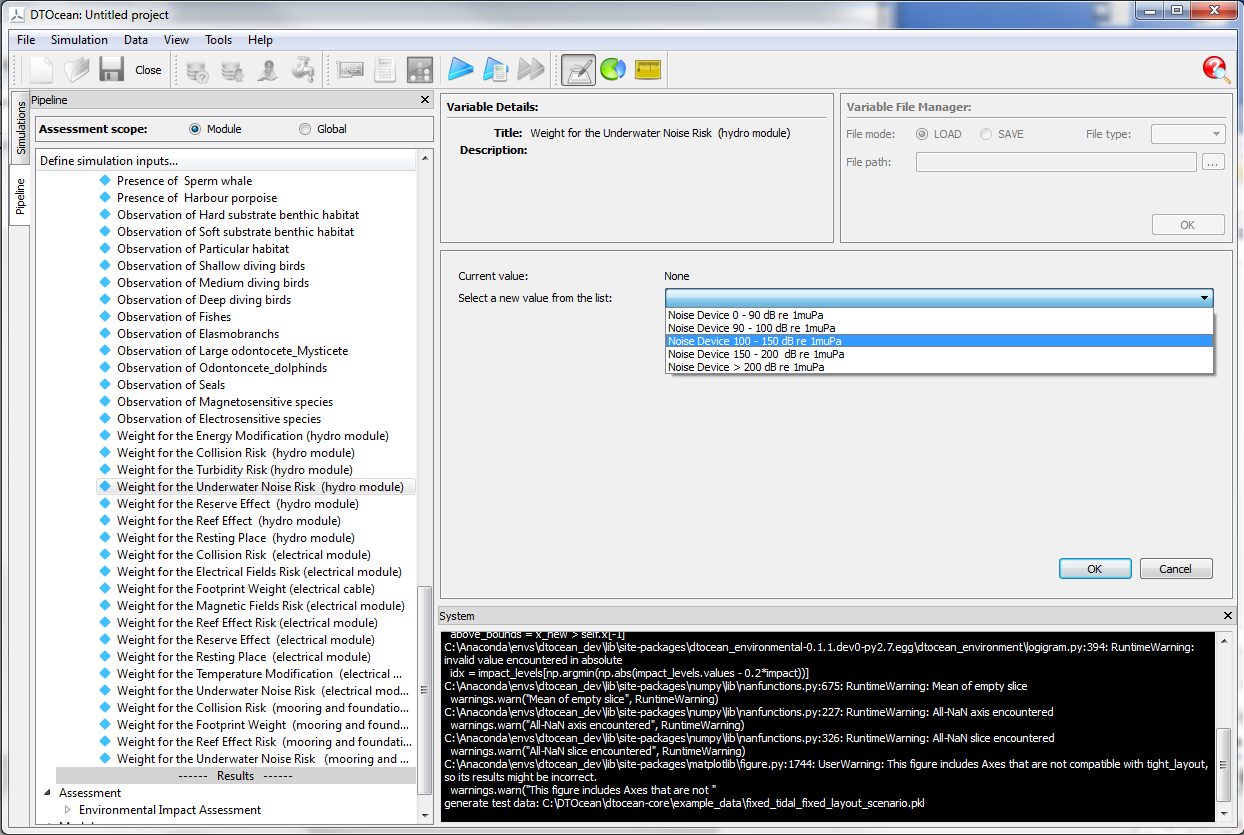
Fig. 7.32 Example of weighting parameters selection for the underwater noise function in the hydrodynamics module.

• STEP 2: Quantification of the receptor sensitivity and STEP 3: Qualification of the seasonal distribution of receptors

The steps 2 (Receptor qualification) and 3 (seasonal distribution) are grouped together in the GUI. For each category of receptor, the user has the following choices:

1. complete the observation box by true, false or a blank box if there is no information.
2. If the selected category of species is supposed to be observed all year long, but the user does not have this precise information, the user can simply complete the first bow called “year” That will lead to a medium confidence level for the EIS score.
3. If the selected category of species is exactly known to be observed all year long, the user has to complete all boxes. That will lead to a high confidence level for the EIS score.

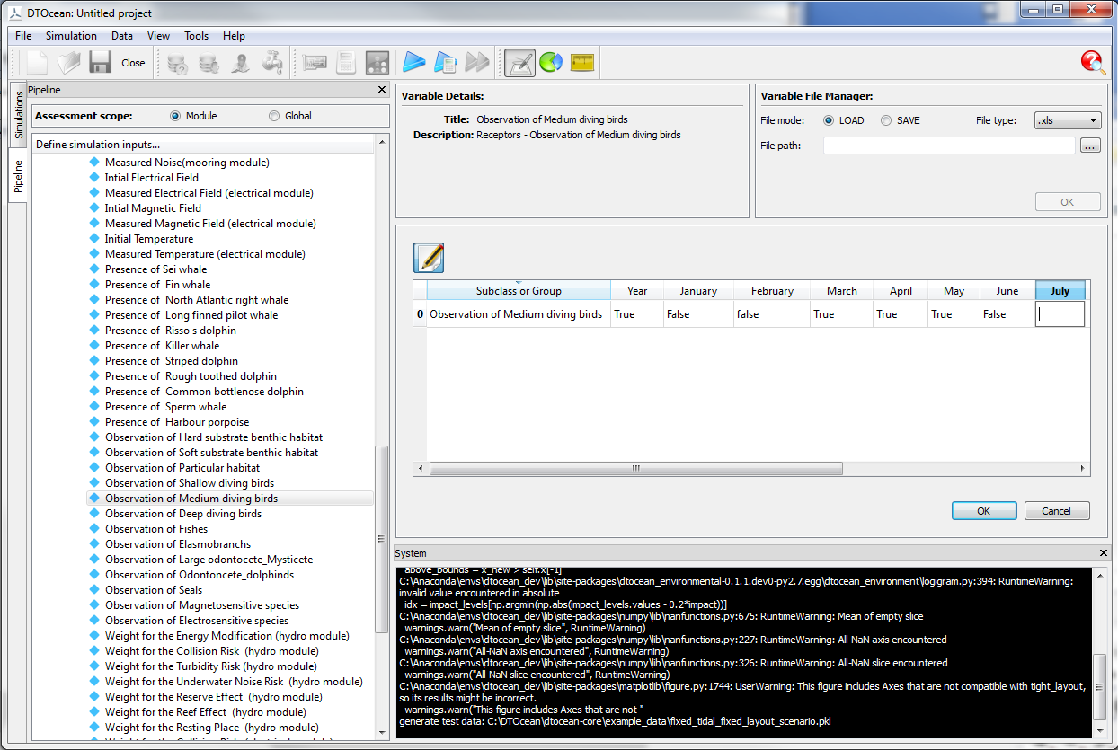
Fig. 7.33 Example of the EIAM GUI for the medium diving birds receptor category

Protected species / “red list”:

In the case where the user want to declare a species included in the “red list”, he has to tick the box in the corresponding line of the receptors list presented in the pipeline as shown in the figure below.

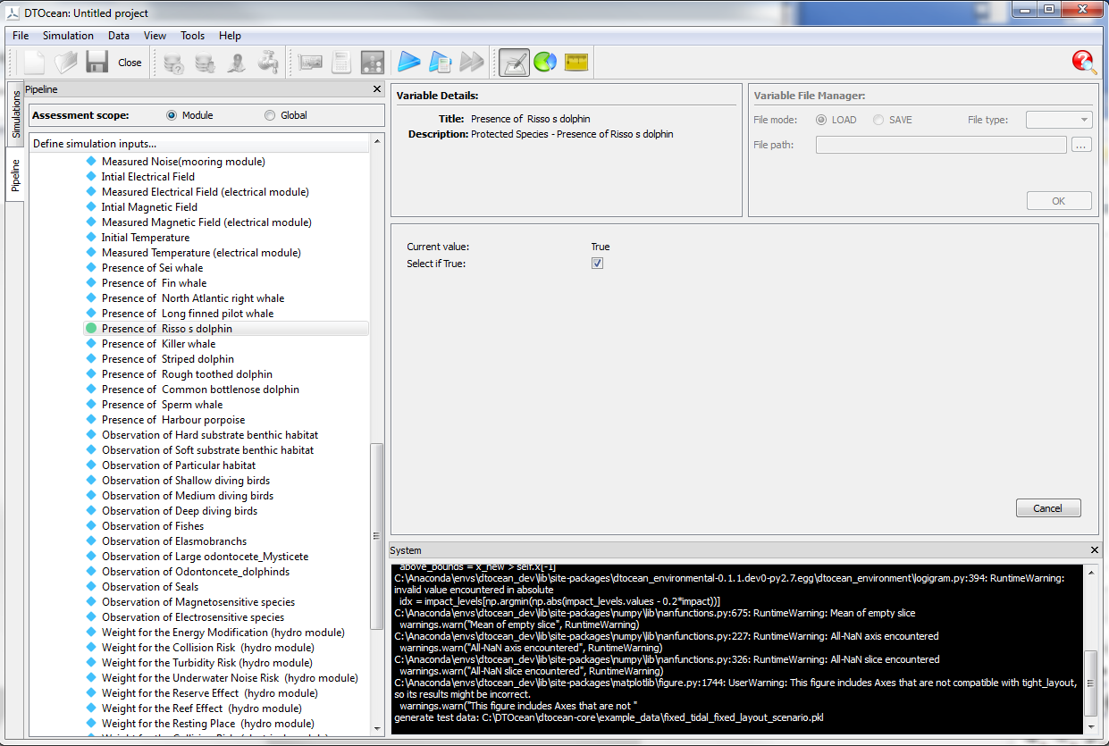
Fig. 7.34 Example of the EIAM GUI for a species of the “red list”: the Risso’s dolphin

7.3.2.3. Outputs

The main outputs from the EIAM will consist of a set of scores. In order for the user to have both a global environmental assessment and detailed information when using the DTOcean EIAM, two levels (L1 and L2) of results are available within the software. At each level, adverse and positive impacts are always given separately. The different display levels are defined as follow:

• Level 1: The first level of assessment provides a global (agglomerated) EIS given for each module. The result for each module is generated by the summation of EIS obtained by each function selected for that specific module and normalised on the scal e ranging from +50 to -100. This level also contains the range of impacts associated with the EIS for each module. A graphical example of the level 1 results is given in Fig. 7.35.

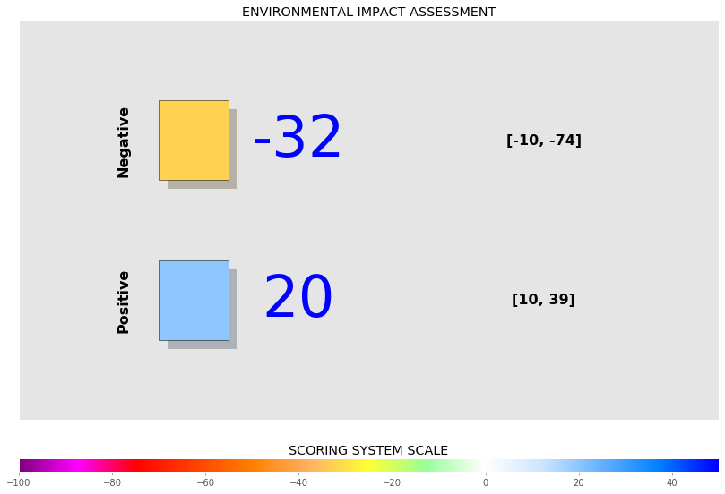
Fig. 7.35 Illustration of the module environmental impact score display

• Level 2: The second level provides full details at the function level. This level also contains the level of confidence associated to the EIS for each function. A graphical illustration of this level is shown in Fig. 7.36.

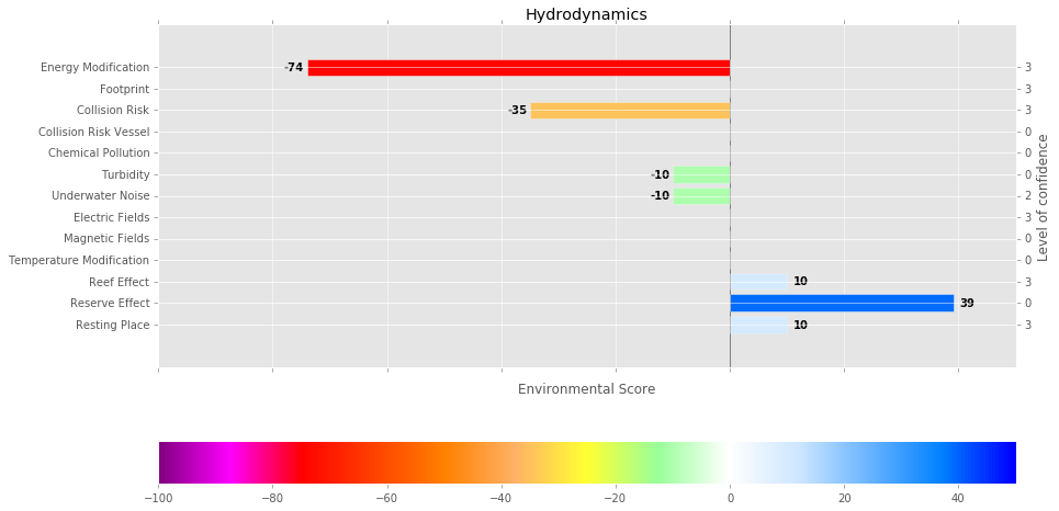
Fig. 7.36 Illustration of the function environmental impact score display

A set of recommendations is also implemented in the EIAM module. Its purpose is to help the user to better understand what lies behind the scores in term of qualitative issues related to the pressure scores. The recommendations are specific and a set of recommendation is available for each function of the modules. They are available through the graphical User Interface (GUI) when EIS are displayed. Examples of recommendations are given in Fig. 7.37 below.

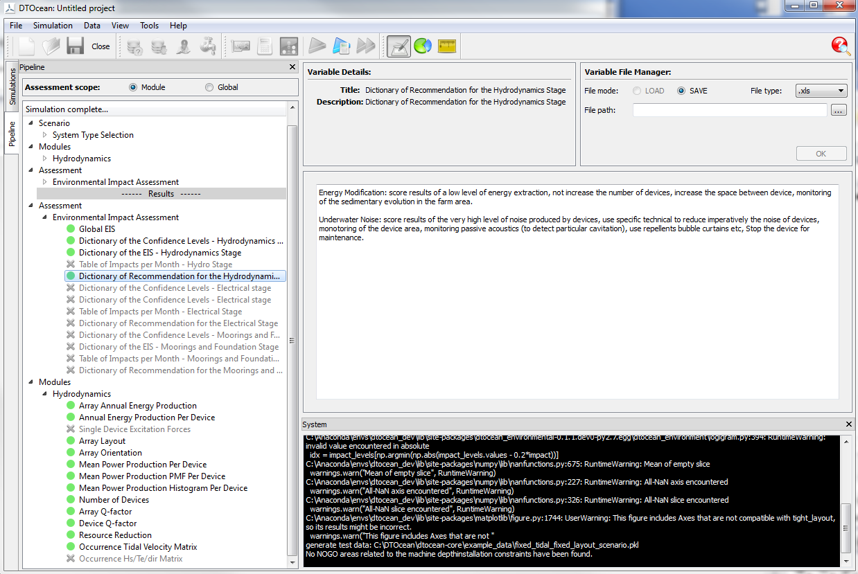
Fig. 7.37 Illustration of recommendations given in the GUI