5. Main Application and Graphical User Interface

5.1. Introduction

The section presents the development of the main application for executing the modules, thematic assessments and solution strategies within the system – along with means to upload and download data, using various sources, and plot results. Also described in this chapter is the graphical user interface which provides a view for controlling the main application.

5.2. DTOcean Core

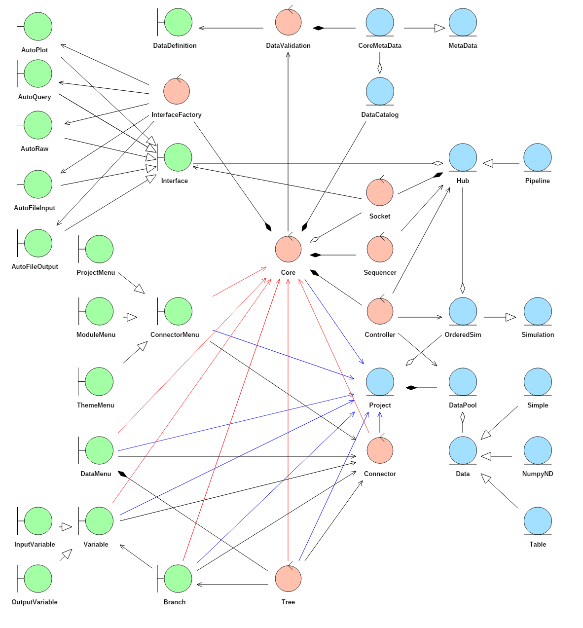
Fig. 5.19 Robustness diagram for the DTOcean Core

5.2.1. Primary Functionality

Objectives

The objective of the DTOcean Core component is to facilitate the execution of packages in the correct manner, and provide a means for the user to control the execution of their associated Python packages and observe and modify the data supplied to and generated by them.

The execution of the external packages and storage and control of the data being sent between them is handled by the Aneris framework with some specific customisations (as described below) to meet the requirements of the DTOcean project. The user interaction with the Core is facilitated using a programmatic model of the DTOcean GUI. This model provides a set of classes that operate like specific components of the GUI itself.

Customisation and Incorporation of Aneris

The Core provides the bridge, or model, for using the GUI to control the functionality found in the Aneris framework. Additionally, certain aspects of the Aneris framework were customised in order to meet the particular technical needs of the project.

The most fundamental customisation is creating a MetaData subclass which will define the metadata fields that can be accessed within the core for each data member. This subclass is named CoreMetaData. The contents of this subclass are not discussed here, but the fields are described alongside the data structures themselves. The data descriptions themselves are collected by configuring a DataDefinition class which stores the address of a directory containing the definition files (in YAML format).

A related and important customisation is extending the number of Data subclasses so that different structures of data can be included in the core. In Fig. 5.19 three examples of generic data structures are shown: Simple stores single valued typed data, NumpyND is for the Numpy package array objects of arbitrary dimension and Table is for the pandas package DataFrame objects. A number of these classes are described in the data structures section, however Data classes can be subclassed as much as required to meet the specific needs of the data. If something is uniquely structured then a unique Data subclass can be created for it. The ambition, nonetheless, is to store the majority of data members within a limited set of generic structures. This will makes the development of plots, file inputs / outputs and database access for these structures less demanding, for instance.

The Core makes use of all the standard Interface subclasses available in Aneris. Additionally there are a group of interfaces that mix the AutoInterface class of Aneris with the standard interfaces. For example, the AutoQuery class allows interfaces to be created automatically in order to access the DTOcean database. The creation of these interfaces is triggered by the existence of certain fields in the data definitions, and the use of Data subclasses that have the special “auto_db” method for accessing tables and columns specified in the data definition. Because there are different ways to store data in the database, subclasses of the generic Data subclasses (like the Simple class) have been created to return data members from specific types of database structures (like a single row from a single column, for instance). Auto interfaces for raw data entry, file inputs and outputs and plotting have been created in a similar manner.

Standard MapInterface subclasses must also be created to connect external packages. These provide the translation of data structures for the local inputs for external packages and also the translation for returning the outputs to the core. RawInterface and FileInterface classes (and there auto variants) are used to collect data members from the user, where appropriate, and QueryInterface classes can be used to send instructions to the database regarding filtering the available data (by site location, OEC device, etc.)

Three specific Hub objects are used within the Core, one to collect information about the specific scenario being undertaken, one to execute and sequence the chosen computational modules (a Pipeline) and one to execute the chosen thematic algorithms.

These Hub objects and the other Aneris components are stored in two main classes, a control class called Core and an entity class called Project. The Project class holds all the data relating to a particular project, such as the Simulation objects and the DataPool, whereas the Core class gives access to the functions of Aneris and holds any objects that would be constant between projects (for this design, the DataCatalog and Hubs are such items). Holding the project (or scenario) data in a single entity makes the logic of saving and loading projects more straightforward as the goal is to serialise all the contents of this class.

All the remaining classes defined within the Core code, and unrelated to Aneris, make use of the Project and Core classes. To see these connections more easily in Fig. 5.19, associations to the Core class are shown in red and associations to the Project class are shown in blue.

GUI Model and Controllers

The DTOcean Core provides a model for which all of the functionality of the GUI design can be accessed programmatically. To do this, a number of “boundary” stereotype classes are created to support the components of the GUI. For instance to recreate the design stages in the GUI the following classes exist:

• DataMenu
• ProjectMenu
• ModuleMenu
• ThemeMenu

The methods of these classes complete actions that can be undertaken in the GUI, for instance the ProjectMenu can be used to create a new Project object using the new_project method.

The DataMenu is used for configuring and activating the database access or for loading test data from specially formatted python files. All the other Menu classes affect actors accessed through interfaces. The ProjectMenu controls the “project” hub which affects interfaces related to the filtering of the database, for instance. The Module and Theme menus work with the “module” Pipeline and “theme” Hub to prepare and execute the modules and thematic assessments. To support these actions which utilise Aneris Hub classes, an additional controller class, named Connector, was created and the shared actions with this class and defined in the ConnectorMenu class from which ProjectMenu, ModuleMenu and ThemeMenu are subclassed.

The next set of boundary classes relate to interacting with the data members themselves and mimic the “pipeline” part of the GUI design. Provided are a Tree, Branch and Variable class, with the Variable class being further subdivided into the InputVariable and OutputVariable classes.

A control class named Tree has been created to access the Branch classes which are created per module or theme interface that have been chosen as part of the project. The Tree also can do some bulk actions on all branches such as reading from the database.

A Branch object will group all the input and output variables for a particular component (such as an external package). It is also responsible for supplying reports relating to the status of the variable. A variable object can only be retrieved from the related branch.

A Variable class allows the user to examine the data contained in a data member, and execute interfaces that are available for that variable such as raw data entry, database access, plots etc.

DTOcean Packages and 3rd Party Libraries

As the core provides the connection between all the external packages which form the DTOcean software, those packages must be made available to the core. The strategy for achieving this is to create an installable Python package for each major component. The list of packages that are used by the core are as follows:

• dtocean-hydrodynamics
• dtocean-electrical
• dtocean-moorings-foundations
• dtocean-installation
• dtocean-operations-maintenance
• dtocean-logistics
• dtocean-economics
• dtocean-reliability
• dtocean-environmental

Additionally, the Aneris and Polite DTOcean packages are required.

The Core requires a number of 3rd party Python libraries for its operation. These include:

• geoalchemy2
• matplotlib
• matplotlib-basemap
• netcdf4
• numpy
• openpyxl
• pandas
• pil
• psycopg2
• pyproj
• pyyaml
• shapely
• xarray
• xlrd
• xlwt

5.2.2. Additional Components

Packages Interfaces

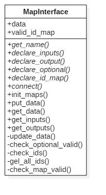
Fig. 5.20 UML Class diagram of the MapInterface class

All computational components in the DTOcean software are developed as installable Python packages or modules that can be executed separately to the main software itself. This provides a number of advantages to the design, in that the packages can be tested independently and also act similarly to any other data coupled component. This structure also allows other, non DTOcean, packages to be interfaced into the software in a similar manner, possibly replacing some functionality in DTOcean with a more complex tool.

The specific method for interfacing with external packages is through an Interface class, as found in the Aneris framework. More specifically, MapInterface sub-classes have been used, as these allow a semantic disconnect between the data member identifier and the identifier used to recover the data to pass into the external package. This disconnect is useful as minimal changes are required if changes are made to the data definitions or external package entry points.

The Aneris framework can also handle inputs to the external packages that are optional. These must be declared by listing the inputs as the return value of the “declare_optional” method. The system will then allow execution of the package if these optional inputs have not been satisfied. Additionally, Aneris MaskVariable classes can be used in the input list to mask inputs until certain criteria are met for another data member.

The UML class diagram for a MapInterface class is given in Fig. 5.20. Note that the first 6 methods are abstract methods, in that subclasses must be created which implement these methods or otherwise an error will occur. Each subclass of MapInterface describes the interface to one particular external package and each of these (when placed in the correct location) can be automatically discovered by Aneris’s Socket class.

The abstract methods which each interface subclass must implement are described below:

• get_name: A method which returns the user readable name of the external package being called. These should be unique
• declare_inputs: A method which returns all of the data member identifiers that are required inputs to the interface as a list of strings and / or MaskVariable objects. The identifiers must match those in the data definitions
• declare_outputs: A method which returns all of the data member identifiers that are outputs from the interface as a list of strings. The identifiers should match those in the data definitions
• declare_optional: A method which returns all of the data member identifiers that are optional inputs as a list of strings. These identifiers declared here are not strictly required for execution of the external package. The identifiers should match those in the data definitions
• declare_id_map: A method which returns the mapping for variable identifiers given in the data descriptions to local names for use in the interface
• connect: A method which is used to execute the external package using inputs collected from the data attribute and then populate the data attribute with values created by the external package

As mentioned above the data attribute of the interface can be used to both access input values and provide output values. In the MapInterface class the data values can be accessed like class attributes, for example to collect the value of the locally named variable “my_variable”, the process is simply to request “self.data.my_variable”.

Data Tools

The potential functionality of the data tools within DTOcean is somewhat broad. There are two key use cases for data tools which are addressed. These are:

• Tools that can manipulate data within interfaces of external packages
• Tools that can manipulate data outside of the tool (for data preparation purposes)

Another desirable feature of these tools is for them to be extensible, in a similar manner to external package interfaces, thus they should be accessed through an Aneris Plugin subclass.

Examples of tools that are used in the DTOcean software include:

• Conversion of time domain environmental data to statistical form
• Conversion of wave period definitions
• Preparation of Hydrodynamic coefficients for wave device modelling

Strategy Manager

The Strategy Manager component of DTOcean provides a flexible framework for developing automated processes in the software, be that for a single complete simulation, sensitivity analysis or more complex optimisation algorithms. It is desirable for this functionality to be extensible such that new execution strategies can be easily integrated into the software.

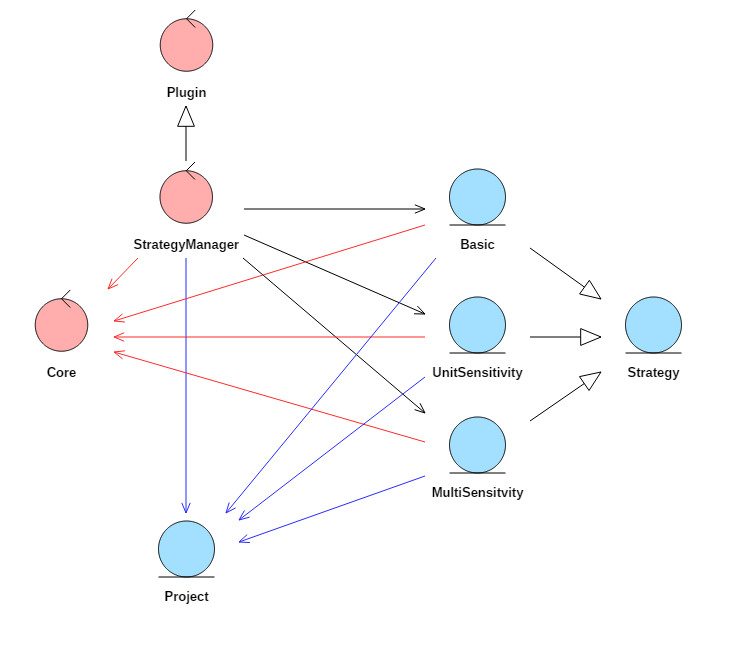
Fig. 5.21 Robustness diagram for the sequencing and optimisation component

A higher level controller for the functionality of the Core is provided, which will be known as the StrategyManager class, as seen in Fig. 5.21. A base class “Strategy” is then provided (following a similar idea to Interfaces) for which a number of abstract methods must be provided in order to define a strategy. Subclasses of the Strategy class can be generalised of to any algorithm used to carry out an automated simulation using the DTOcean software. The Strategy classes utilise the same set of standardised boundary methods, used to interact with the Core and active Project classes, as the user.

The StrategyManager class uses the Aneris Plugin functionality to discover Strategy classes. This allows the user to select which Strategy class they wish to use, and also configure its behaviour.

With this architecture the user can design advanced learning strategies which could leverage existing optimisation packages written for Python. Such packages include:

• Scikit-learn
• Mystic
• DEAP
• cma

5.2.3. Functional Specification

This section describes the operation of the core without the use of the GUI.

Data Lifecycle

A key feature of the Aneris framework (and, thus, of the DTOcean Core) is the strict contracting of data used within the core and exchanged with the external packages interfaced with the Core. This contracting ensures that a single unified definition for the meaning and structure of a piece of data is stored within the core. Interfaces to external components can then be used to deliver and collect the required data, translating from the local representation of that data into the global representation within the core. Four items must be prepared to establish the contracts for the data. These are:

• Defining the data structures
• Defining meta data fields
• Defining data definitions (DDS)
• Defining interfaces

Defining Data Structures

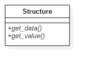
Fig. 5.22 UML Class diagram of the Data class

The Structure class shown in Fig. 5.22 must be the superclass of all data structures defined within the core. For every Structure object two abstract methods must be provided: “get_data()” which prepares data to be stored within the core and will check that the data has the correct structure; and “get_value()” which returns a copy of the data stored with the core in the expected format.

Various Structure subclasses can be provided to provide storage for different structures of data which can validate the raw data being entered into the Structure object from an interface.

Listing 5.1 Python code for the DateTimeData class

class DateTimeData(Structure):

   '''A datetime.dateime data object'''

   def get_data(self, raw, meta_data):

      if not isinstance(pydatetime, datetime):

         errStr = ("DateTimeData requires a datetime.datetime
                   object as ""raw data.")
         raise ValueError(errStr)

      return raw

   def get_value(self, data):

      return data

Listing 5.1 shows an example of a data structure class, in this case for storing a date as a Python datetime.datetime object. The class contains a basic check that the raw data being added meets the expected structure. A further advantage of defining each data structure is that the other parts of the software can respond automatically to various structures. For instance, appropriate plots or file inputs / outputs can be provided based on the data structure of a data member. To define a plot for a structure, for example, the user would add the static method auto_plot to the Structure definition. Once placed in the “definitions.py” file within the data submodule of the core, the data structure subclasses are discovered automatically by the Validation class of Aneris, allowing easy inclusion of new classes as required.

Defining Meta Data Fields

Listing 5.2 Example data definition in YAML format

- description: 'Tidal: represents the position of the hub.
                Wave: represents the position of the centre
                of gravity of the whole device or the point
                of rotation.'
   identifier: device.coordinate_system
   label: Position of the local coordinate system
   structure: NumpyND

Upon installation of the code, any definitions for the data within the Core must be written in YAML format and placed within the “yaml” folder of the data submodule. An example of a definition given in this format is shown in Listing 5.2.

Creating and editing the definitions in YAML format when the amount of data in the project is very large can be somewhat arduous. To make this workflow more efficient some special helper scripts were added to Aneris to allow conversion from Microsoft Excel format files to the YAML format. This function is available on the command line and is called “bootstrap_dds”. It will convert all the Excel files found in a given folder to YAML format and save these in the desired destination folder.

Defining Interfaces

The interface definitions are the most complex part of the data lifecycle of the DTOcean software. Partly, this is because there are a significant number of them. Different interfaces are available for:

• The external packages
• Collecting / providing data from / to the user using files or in raw Python objects
• Communicating with the database
• Creating plots

To help distinguish which interfaces should be grouped together, some subclasses of the interface classes defined by Aneris have been created in the core. One of the first actions to be completed with the software is to contact the database for the top level project data and a special QueryInterface subclass called ProjectInterface is provided for this purpose. The external packages require distinct interfaces so they have subclasses of the MapInterface called ModuleInterface and ThemeInterface respectively. Although, a number of automatically generated interfaces are included for collecting raw data from the user, defining database access, plots, etc., there may also be the need (particularly for plots) to create bespoke interfaces that can, for instance, plot many data members in the same plot.

The most complex interfaces to design are those for the external packages. The interfaces are descendants of the MapInterface, details of which is given in the Aneris description. Listing 5.3 shows a simplified example of the interface for the Hydrodynamics module. Note that identifiers in the input and output list must correspond to identifiers in the data definitions. Additionally, each identifier must have a local mapping given in the id_map dictionary.

The connect method, which is used to call the code of the external package (in this case for the Hydrodynamics module,) has access to the data defined in the interface through the attribute “self.data”. Each variable name defined in the local mapping can be accessed or written to through this variable using simple “dot” notation as can be seen in Listing 5.3.

The local mapping also allows changes in the data definitions to be isolated from changes in the external package definitions. Such a change would require simply a two line alteration in the interface, changing the input or output id and the id_map dictionary.

Listing 5.3 Simplified interface for the Hydrodynamics module

class HydroInterface(ModuleInterface):


   def __init__(self):

      super(HydroInterface, self).__init__(weight=1)

   @classmethod
   def get_name(cls):

      return "Hydrodynamics"

   @classmethod
   def declare_inputs(cls):

      input_list  =  ["bathymetry.depth",
                     "farm.hydrodynamic_folder_path"]

      return input_list

   @classmethod
   def declare_outputs(cls):

      output_list = ["farm.annual_power"]

      return output_list

   @classmethod
   def declare_optional(cls):

      optional = ["farm.hydrodynamic_folder_path",
                 ]

      return optional

   @classmethod
   def declare_id_map(self):

      id_map = {"bathymetry": "bathymetry.depth",
                "hydro_folder_path": "farm.hydrodynamic_folder_path",
                "AEP_array": "farm.annual_power"}

      return id_map

Initialising the Core and Database Access

The DTOcean software is designed to operate alongside a database containing stored data for multiple scenarios (a scenario being a combination of data relating to a single development site and a single energy conversion technology). The purpose of this database is to reduce the data entry burden on the software user, by providing a baseline data set prior to beginning the operation of the core. Of course, correctly formatted data must be entered into the database in order to make it available to the core, but this is a onetime operation versus re-entering the data into the core upon each usage.

The core treats the database as an understood structure, in a not necessarily understood location. The default location for the database is locally hosted next to the DTOcean software, but the core is capable of connecting to similar databases on local networks or even remote networks, however data retrieval times will obviously increase as the distance to the database increases. It is important to note that the database may not be used with multiple parallel sessions of DTOcean, i.e. it is single user only.

Listing 5.4 Example of database location description in YAML format

"local":
   host: "localhost"
   dbname: "dtocean_base"
   schema: "production"
   user: "yourusername"
   pwd: "yourpassword"
"remote":
   host: "555.555.555.555"
   dbname: "dtocean_shared"
   schema: "clone"
   user: "guest"
   pwd: "guest

Database addresses are specified in a configuration file located in the AppData folder for DTOcean (for instance: C:UsersYourUserNameAppDataRoamingDTOceandtocean_coreconfig) in a file named database.yaml. Listing 5.4 gives an example of specifying a database location for a locally stored and remote database. Note PostgreSQL schemas can be used to allow multiple versions of the database tables to be used within a single database, making cloning more straightforward.

Listing 5.5 Creating a Project and connecting a database

my_core = Core()
project_menu = ProjectMenu()
data_menu = DataMenu()

my_project = project_menu.new_project(my_core, "Test")
data_menu.select_database(my_project, "local")

Setting up a project and connecting a database is demonstrated in Listing 5.5. An instance of the Core, ProjectMenu and DataMenu classes are required and then a Project class can be created. Associating the desired database to the project is then done through the DataMenu´s select_database method, giving the project and the name of the definition in the YAML file as inputs. The updated project is then returned.

Mapping particular data members to locations within the database structure is achieved through definitions given in the DDS files and special methods within the data structure definitions called “auto_db”.

Listing 5.6 Example of a Structure subclass implementing an “auto_db” database access method

@staticmethod
def auto_db(self):

   if self.meta.result.tables is None:

      errStr = ("Tables not defined for variable "
                "'{}'.").format(self.meta.result.identifier)
      raise ValueError(errStr)

   Table = self._db.safe_reflect_table(self.meta.result.tables[0])
   result = self._db.session.query(
                  Table.columns[self.meta.result.tables[1]]).one()

   self.data.result = result[0]

   return

Listing 5.6 gives an example of a subclass of a data structure which implements an auto_db method. The method works on a list of strings, provided in the “tables” field of the DDS meta data, that refer to particular locations in the database. The first entry will always be a table name, but later entries could have various meanings depending on the context. In the method is a special local data reference called “result” which is used by the core to retrieve the result of the database query when data structures with auto_db methods are discovered.

The auto_db methods provide fine control of database access but larger scale filtering operations can also be carried out using the QueryInterface class of Aneris. This interface provides access to the database object stored within the core which can be used to implement stored procedures within the database, given a particular set of input values (specified in an identical manner to those for the external package interfaces). This methodology is used for filtering multiple sites and technologies stored within the database to single selection and their associated data.

External Package Execution

The main burden for executing an external package with the DTOcean software lies in specifying the necessary inputs for that package to run. However, as the system can run with multiple packages the number of required inputs for a package may vary. Therefore, it is necessary to inform the core about database selections and how many packages are desired to compute before beginning the data collection task. The process is shown in Fig. 5.23 and, to summarise, following opening a project, the user must:

1. Connect a database and filter it for project data if desired.
2. Activate external packages for execution
3. Examine which inputs must be satisfied to execute the first package
4. Enter inputs into the core and test if the all the inputs have been provided
5. If so, execute the package

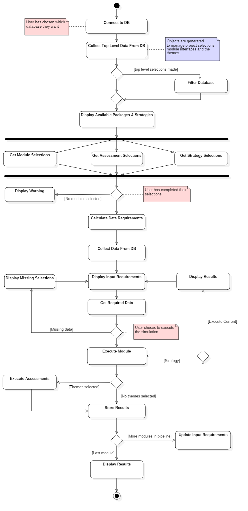
Fig. 5.23 Activity diagram for executing external packages

Activating Computational Modules and Thematic Algorithms

Assuming that a database not been selected, the first requirement for external package scheduling is to initiate the “pipeline”. This initiates the inbuilt hubs and pipelines required for filtering the database and activating and scheduling the packages. It also collects data that can be used as filters for the database, by selecting a site and technology from the retrieved lists. This command is used as follows:

project_menu.initiate_pipeline(my_core, my_project)

It is possible to retrieve the names of the computational modules which can be scheduled from the core. The command and sample output are shown in Listing 5.7. This functionality is provided by the ModuleMenu class

Listing 5.7 Retrieving the available module names

module_menu = ModuleMenu()
names = module_menu.get_available (my_core, my_project)

“names” content:

Hydrodynamics Electrical Sub Systems Mooring and Foundations Installation Operations and Maintenance

Activating a computational module, for instance the Hydrodynamics module, is then achieved by issuing the command:

module_menu.activate(my_core, my_project, 'Hydrodynamics')

It is important to ensure that the name given in the final argument of the activate command matches one of those names given by the get_available command seen in Listing 5.7.

Any number of computational modules can then be activated, although each available module can only be activated once. The order of execution is strictly controlled in the core in order to ensure that the interrelationships between the computational modules are adhered to.

In a similar manner the thematic algorithms can be checked and activated using the get_available and activate commands from the ThemeMenu class.

Satisfying Inputs

In order to inspect the status of the inputs for an external package, a Branch class associated to the package must be created. Naturally, to get a branch, first you need a Tree, and the example for getting the branch for the Hydrodynamics module is as follows:

my_tree = Tree()
hydro_branch = my_tree.get_branch(my_core, my_project, "Hydrodynamics")

The status of the inputs required for the Hydrodynamics module is retrieved using the following command shown in Listing 5.8, and an example of the content is shown there also.

Listing 5.8 Retrieving the input status of the Hydrodynamics module and its contents

input_status = hydro_branch.get_input_status(my_core, my_project)

   farm.main_direction: optional
   farm.user_array_option: required
   device.power_rating: required
   device.minimum_distance_x: required
   device.minimum_distance_y: required
   device.installation_depth_min: required
   farm.geophysics: required
   farm.blockage_ratio: required
   device.coordinate_system: required
   farm.rated_power: required
   device.installation_depth_max: required
   farm.power_law_exponent: required
   farm.selected_technology: required
   device.floating: required
   farm.user_array_layout: optional
   bathymetry.depth: required
   farm.lease_boundary: required

The input status of a branch is a Python dictionary with keys that match identifiers found in the DDS and values that relate to the data needs of the package in order to be able to execute. There are five possible values that this status can have, described as:

• required: The data is necessary to execute the package and has not been entered into the core
• optional: The data can optionally be entered into the package, but has not been entered into the core
• satisfied: Necessary or optional inputs to the package that have been entered into the core
• unavailable: Inputs to the package that will be overwritten by another package executed before the one being inspected
• unavailable_option: Optional inputs to the package that will be overwritten by another package executed before the one being inspected

Entering Inputs

Once it has been established which inputs are required to execute one or all of the computational modules the necessary or optional data must be entered into the core. In general, this can be achieved using Interface classes, which facilitate collecting inputs directly from the user, from the database or from files.

Within the DDS database mappings for various data members can be defined and these are retrieved using the auto_db methods defined within the data structures. If we wanted to attempt to collect the data for a single variable from a database, for example the farm.main_direction variable of the hydrodynamics branch, then the commands are:

new_var = hydro_branch.get_input_variable(my_core,
                                          my_project,
                                          "farm.main_direction")
new_var. read_auto(my_core, my_project)

Then the new value for the variable will be loaded into the project. Obviously, it would be a slow process to do this for every variable, so the user can apply the read_auto method to every valid variable in the branch, by issuing the command:

hydro_branch. read_auto(my_core, my_project)

Assuming some inputs could not be retrieved from the database, or the user wishes to override some of them, then other interfaces can be used to collect data. The most common is the RawInterface, which collects data directly from the user in the form of Python objects. The core will automatically create raw interfaces for all variables.

Providing a raw input to a variable is very similar to the process for retrieving data from the database. Again, setting the farm.main_direction variable to 180 as an example, the process would be as follows:

new_var = hydro_branch.get_input_variable(my_core,
                                          my_project,
                                          "farm.main_direction")
new_var.set_raw_interface(my_core, 180.)
new_var.read(my_core, my_project)

Note that set_raw_interface is checking to see if there is a unique interface defined for the variable. This is always the case for raw inputs but may not be for file interfaces, for instance, where several different formats could provide the same data. To examine which file interfaces are available for inputting a variable the user issues the get_file_input_interfaces command like so:

new_var = hydro_branch.get_input_variable(my_core,
                                          my_project,
                                          "farm.geophysics")
file_interfaces = new_var. get_file_input_interfaces(my_core)

The file_interfaces variable now contains a list of file interface names that can be used to retrieve the data. Once one is chosen from this list, it can be activated in a manner similar to the following:

new_var.set_file_interface(my_core, "path/to/my/file.xyz", "GeoXYZInterface")
my_project = new_var.connect

The above processes should be repeated until all the necessary inputs and desired optional inputs are satisfied. Finally, to check if the computational module can be executed, the following command will return True or False:

module_menu.is_executable (my_core, my_project, "Hydrodynamics")

Executing the Computational Module(s)

If the result of the is_executable test for the next executable module is “True” then the computational module can be safely executed. This is done as follows:

module_menu.execute_current(my_core, my_project)

The computational modules will always run without requiring interaction from the user. Also, any activated thematic algorithms will be executed automatically following completion of the module, assuming the necessary data to run the theme has been produced.

Selecting and Executing a Strategy

Another option for executing computational modules is using a Strategy class, for either a simple simulation containing all the available modules, or more complex sensitivity and optimisation studies. Selecting a strategy involves the use of a StrategyManager as follows:

strategy_manager = StrategyManager()

unit_strategy = strategy_manager.get_strategy("Unit Sensitivity")

The list of available strategies can also be recovered from the StrategyManager with the command “get_available_strategies()”. Once a strategy has been selected it must be configured and then executed. Configuration varies from strategy to strategy but the methods that must be called are always the same. Configuring and executing the strategy selected above is implemented using:

unit_strategy.configure("Hydrodynamics",
                        "farm.rated_power",
                        [5, 10, 20])
unit_strategy.execute(my_core, my_project)

The configuration of this strategy will run 3 simulations where the farm rated power is varied for the as an input to the hydrodynamics module between 5, 10 and 20MW.

Inspection of Results

Following completion of an external package, the results are presented to the user in a similar manner to which the input data was collected. Firstly, the status of the outputs can be found using the same Branch object that was used to show the status of the inputs. As an example, the command to get the output status for the Hydrodynamics module and the content of that variable are shown in Listing 5.9.

Listing 5.9 Retrieving the output status of the Hydrodynamics module and its contents

output_status = hydro_branch.get_output_status(my_core, my_project)

   farm.annual_power_per_device: satisfied
   farm.layout: satisfied
   farm.annual_power: satisfied
   farm.mean_power_per_device_per_state: satisfied
   farm.number_of_devices: satisfied

Similarly to the input status, the output status of a branch is a Python dictionary with keys that match identifiers found in the DDS. Here, the values relate to the data associated to the identifier: whether it exists and whether it was created by the external package associated to the branch. There are three possible values that this status can have described as:

• unavailable: The data associated to this identifier has not been entered into the core
• satisfied: The data associated to this identifier has been entered into the core by the package associated to this branch
• overwritten: The data associated to this identifier has been entered into the core by a package which has executed after the package associated to this branch

Recovering the value of the data generated by the external package requires the user to retrieve the OutputVariable object for the given variable identifier and then extract the raw data from that object.

For instance, to get the value of the number of OEC devices produced by the Hydrodynamics module, the process is as follows:

n_devices = hydro_branch.get_output_variable(my_core,
                                             my_project,
                                             "farm.number_of_devices")
value = n_devices.get_value(my_core, my_project)

It is also possible to generate charts using just the data contained in a single OutputVariable object. Because the metadata associated to the identifier is contained inside the object, descriptive information is used to decorate plots. Fig. 5.24 shows how such as chart can be created, for the annual power production per device output of the Hydrodynamics module.

annual_power_per_dev = hydro_branch.get_output_variable(my_core,
                                          my_project,
                                          "farm.annual_power_per_device")
annual_power_per_dev .plot(new_core, new_project)

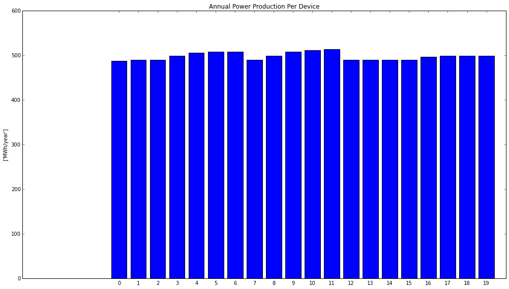
Fig. 5.24 Creating a chart using a single OutputVariable object and the matplotlib library

5.3. Graphical User Interface

The graphical user interface (GUI) must facilitate the implementation of the core, optimisation and data tools components. This section presents the technical implementation of the GUI design.

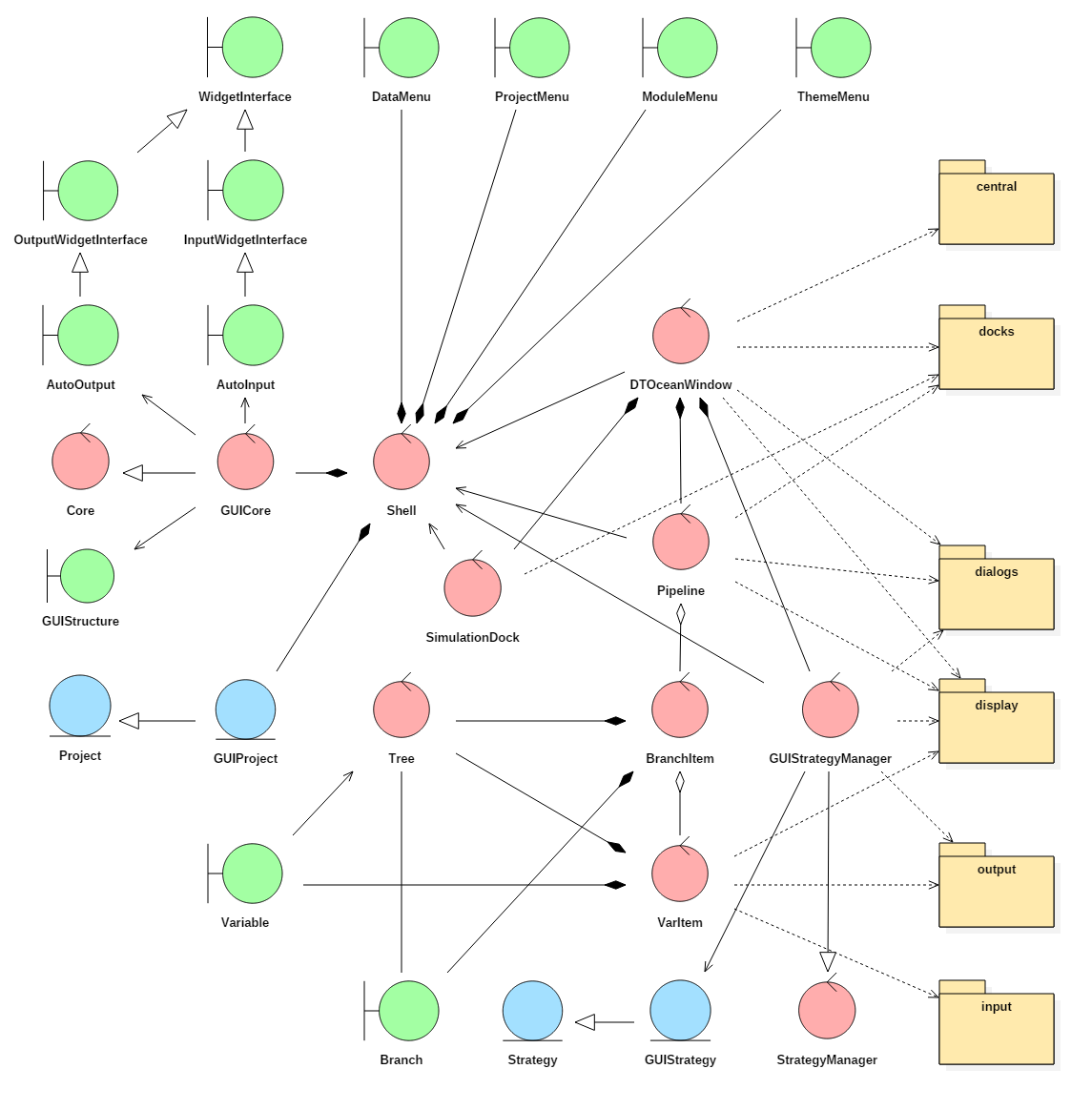
Fig. 5.25 Robustness diagram for the graphical user interface

The GUI design in specified seven main features:

• A main window with menus
• A docked area for recording / switching Simulations
• A docked area for the “pipeline” which displays variables triggers displays
• An textual input collection / output display area
• A graphical display area
• A simulation comparison area
• A log window dock
• Various pop-up dialogues

These components are created using the Qt4 framework and are converted to Python compatible code using the PyQt package. Once created with PyQt they can be modified and manipulated dynamically with the requirements of the software.

These widgets (the common name in Qt for an isolated graphical object) are stored in Python modules related to their purpose, as is seen in Fig. 5.25. As required the control classes of the GUI can subclass these widgets and use their display and signalling capabilities.

The main classes related to the operation of the core, the Core control class and the Project entity class, are subclassed into the classes GUICore and GUIProject in order to allow signally of events to be triggered when changes are detected. These subclasses are then stored in another class named “Shell”. This is a technicality for sharing a single instance of these classes between the various parts of the GUI which will remain synchronised. The boundary classes related to menus (DataMenu, ProjectMenu, ModuleMenu and ThemeMenu) are also stored within the Shell class.

To provide a logical distinction of the various purposes of the GUI, four additional control classes are provided. The “DTOceanWindow” class is responsible for setting up the main window of the software, supplying menu options, generating new docks and spawning pop-up dialogues as required for various purposes. To facilitate this it contains the three other main control classes

The “Pipeline” class is responsible for creating the main interactive component of the software, building the dock which contains the pipeline, input / output, display and system information areas of the GUI. The Pipeline class contains a Tree class so that it can build the branches of pipeline which relate to the external packages connected to the DTOcean software. The Pipeline class can generate many types of children classes, but only two of these are discussed here.

A “BranchItem” class allows per interface operations to be completed as a group - this includes updating the input / output statuses, for instance. Branches are also responsible for creating “VarItem” subclasses related to the branch.

“VarItem” subclasses are used to provide functionality relating to the variables themselves, either inputs or outputs. This includes selecting the correct input, output and display widgets; feeding data to and from these widgets and the core; displaying the input / output status to the user. They also trigger the current display to update either its data or plot depending on which context area is selected.

The other main control classes are the SimulationDock class which manages active simulations within the current project and allows for cloning and renaming of those simulations. Finally, the GUIStrategyManager is a subclass of the StrategyManager which provides a dialog for choosing a strategy. It discovers GUIStrategy classes which are subclasses of the core’s Strategy class. These subclasses of strategies defined in the core are used to provide a widget that can be used to configure the strategy before execution.