6. DTOcean Modules

6.1. Array hydrodynamic module

6.1.1. Introduction

The scope of the Hydrodynamics module is the identification of an array configuration that maximise the annual energy production (AEP) of the array, while holding the average q-factor of the array above a user specified threshold. The q-factor is an energy losses index, definable as the modification of the absorbed energy due to the hydrodynamic interaction between bodies. It is calculated as the AEP of the array (\(AEP_{array}\)) over the AEP of the same array without considering the interaction.

\[q = \frac{AEP_{array}}{AEP_{WEC} \times N_{WEC}}\]

where \(AEP_{WEC}\) is the energy production of the WEC at the same location, but without interaction with other devices and \(N_{WEC}\) is the number of devices installed in the array.

The package solves the hydrodynamic interaction between the devices in the array and, based on the solution of the hydrodynamic problem, the energy extracted by each device. The latter is in turn used to estimate the q-factor for the array.

The AEP is used as the cost function of the optimisation loop that needs to be maximised. The optimisation parameter space is defined by the array parameters, such as device inter-distance, rows and columns angles, etc.

The optimum search is constrained by the following variables:

• no-go areas
• minimum distance between devices
• maximum number of devices
• q-factor.

No-go area identifies a zone of the lease area where the installation of the device is not possible, in relation to several reasons such as: nfeasible water detph, environmental motivations, etc. The no-go areas are specified by the user, if known a priori, as well as internally calculated based on the site and machine specification.

The minimum distance between devices identifies the minimum allowed distance between installed devices. This distance is constrained by physical limitation, such as vessel operating, but also by theoretical limitation of the numerical model. For example, for an array of WEC, the minimum distance between devices is obtained by the diameter of the inscribing cylinder.

The maximum number of device is used to obtain an array that fits the target array size specified by the user.

6.1.2. Architecture

The core of the package is divided into two sub-packages, namely tidal and wave.

The tidal sub-package solves the hydrodynamic interaction between turbines using a parametrised look-up table to describe the wake shape and solving the wake interaction based on the semi-empirical models inherited from the wind sector. The wakes are placed in the array area based on the estimation of the streamlines evaluated using Lagrangian drifters at the turbines locations. The wake shape look-up table is populated from CFD runs.

The wave sub-package solves the hydrodynamic interaction within the array using the so-called direct matrix method. The method uses the cylindrical coordinate description of the wave filed generated by the presence of the moving device, and maps it to the global array coordinate system. The solution of the hydrodynamic problem in the cylindrical coordinate system is obtained by solving the Laplace equation in the fluid domain, using a boundary element method solver.

For a detailed description of the mathematical formulation of the hydrodynamics algorithms see (Silva, et al., 2015)

At a high level the hydrodynamics module is divided into two blocks:

• main routine where the pre-processing is carried out
• optimisation routine where the actual array optimisation is performed.

The top-level view of the code is simplified in Fig. 6.1. The figure shows two main and separated blocks: the hydrodynamic module and the wec-standalone module.

The wec-standalone module is a separated module used to generate the input requried by the hydrodynamic module in terms of single machine hydrodynamic for the case of WEC.

The wec-module is not part of the following description.

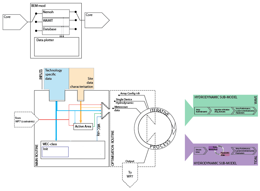
Fig. 6.1 Hydrodynamic model top level view.

The main routine collects the inputs and evaluates the following quantities:

• Assess the No-Go zones from the site bathymetry and installation constraints specified by the users.
• Active Area defined as the lease area subtracted from the no-go areas. The subtraction should be intended as a boolean operation.
• Load the WEC hydrodynamic module genrated by the wec-standalone module.

Additionally, the routine generates three objects; a Hydro, an Array and a Device class object:

• The Hydro class object collects the metocean conditions that describe the features of the site., i.e bathymetry, sea state description, etc.
• The Array class object is used to generate the grid layout given the array type and the parameters value, and to identify which devices are inside the active area. A check on the minimum distance constraint is performed too.
• The Device object collect all the information of the single device and generates all the quantities needed to solve the hydrodynamic interaction between devices.

The optimisation routine calls either the tidal or wave submodule, for the resolution of the array interaction problem, given the required inputs.

6.1.3. Functional specifications

6.1.3.1. Inputs

The hydrodynamic module requires slightly different inputs for arrays of wave and tidal converters as shown in the figure below and detailed in Fig. 6.2.

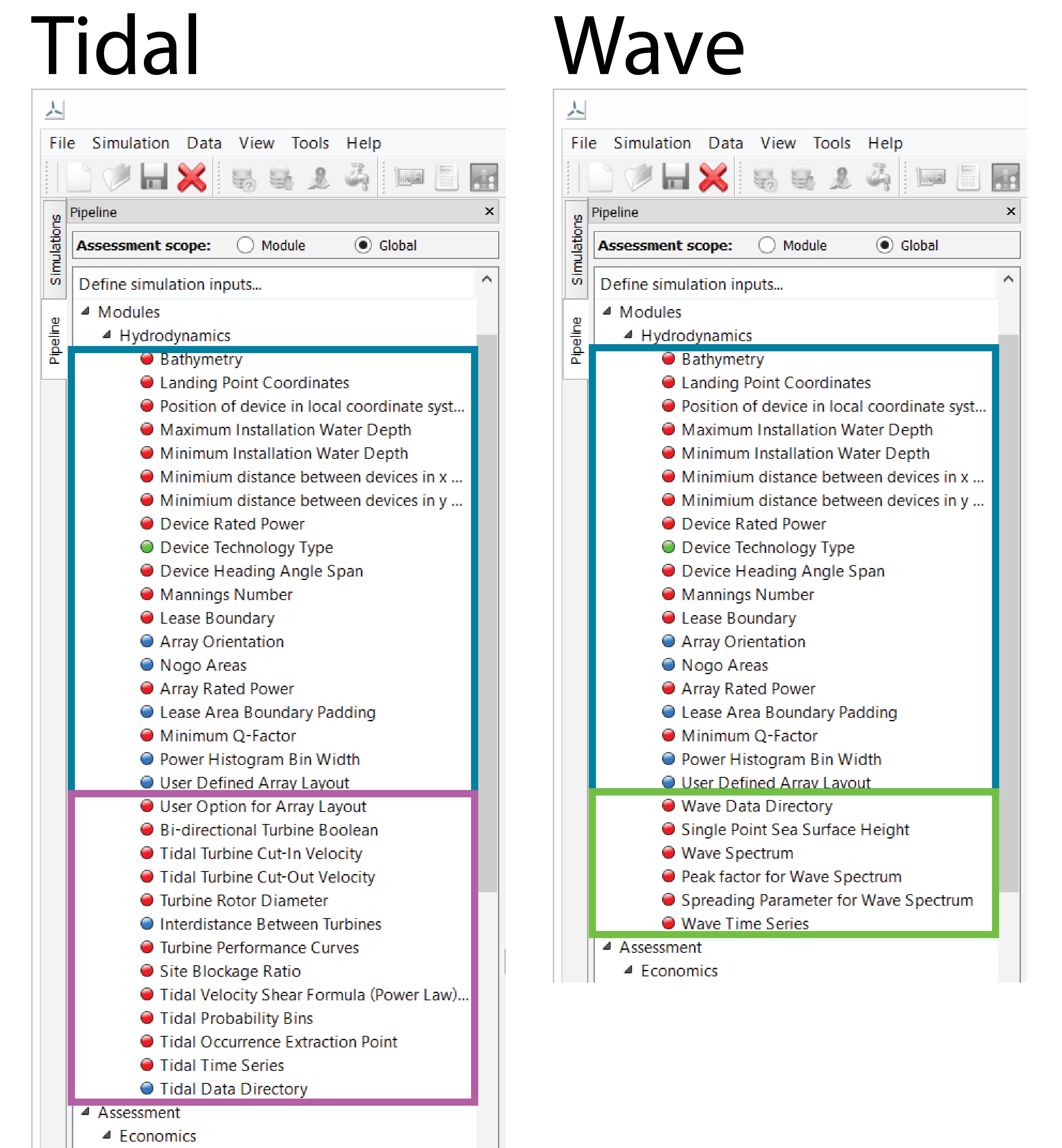
The cyan box represent the common inputs, the purple box the tidal specific inputs and the green box the wave specific inputs. The Red indicator means “missing input”, the Blue “optional input” and the Green “satisfied input”.

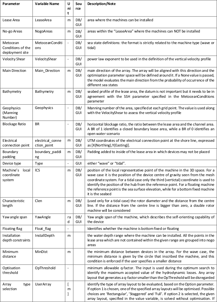
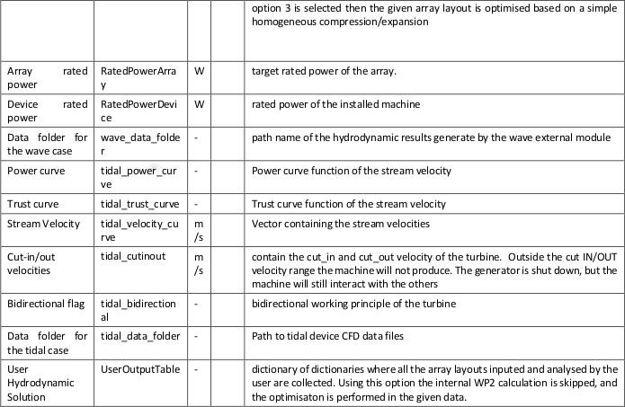
Fig. 6.2 List of inputs for Hydrodynamic module

6.1.3.2. Execution

Once a new project is created the first operation to perform is the selection of the device type. Fig. 6.3 show the four possible choice, the selection is concluded by pressing the Ok button.

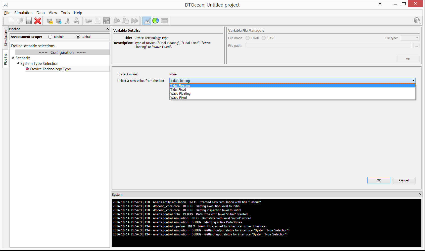
Fig. 6.3 Selection of the device type in the new project input

After the device type is selected, it is possible to add the hydrodynamic module to the list of module to run.

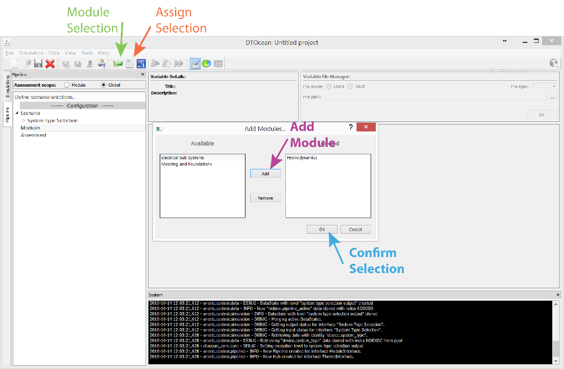
Fig. 6.4 Module selection in the project window.

To perform the operation:

• click the Module Selection icon in the Tool bar (green text and arrow in Fig. 6.4). This will open the Add Module widget.
• Select the Hydrodynamic module form the list of available modules, and click the Add button (purple text and arrow in Figure 5 3).
• confirm the selection by clicking the Ok button (cyan text and arrow in Fig. 6.4).

Prior to perform the last step check if the Hydrodynamic module has been added to the Selected list, otherwise repeat the second step.

After the dataflow has been checked, the user will now be able to add the relevant input for the case to be solved (Fig. 6.5). It is important to note that the data can be inserted manually or using a precompiled database (SQL format).

Once all the compulsory data has been inserted in the GUI, it is possible to run the Module by clicking the Run button in the tool bar.

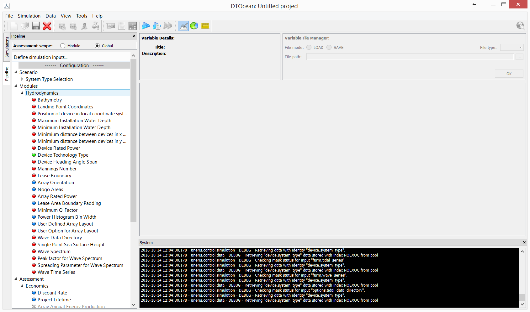
Fig. 6.5 Data Input phase

6.1.3.3. Outputs

As introduced previously the Hydrodynamic module will return an output object at the end of the run with the following attributes (use the GUI visualise manager to plot the relevant data):

• AEP_array (float)[Wh]: annual energy production of the whole array
• power_prod_perD_perS (numpy.ndarray)[W]: average power production of each device within the array for each sea state
• AEP_perD (numpy.ndarray)[Wh]: annual energy production of each device within the array
• power_prod_perD (numpy.ndarray)[W]: average power production of each device within the array
• Device_Positon (numpy.ndarray)[m]: UTM coordinates of each device in the array. NOTE: the UTM coordinates do not consider different UTM zones. The maping in the real UTM coordinates is done at a higher level.
• Nbodies (float)[]: number of devices in the array
• Resource_reduction (float)[]: ratio between absorbed and incoming energy.
• Device_Model (dictionary)[WAVE ONLY]: Simplified model of the wave energy converter. The dictionary keys are:
  • wave_fr (numpy.ndarray)[Hz]: wave frequencies used to discretise the frequency space
  • wave_dir (numpy.ndarray)[deg]: wave directions used to discretise the directional space
  • mode_def (list)[]: description of the degree of freedom of the system in agreement with the definition used in WAMIT taking in consideration only translational degrees of freedom
  • f_ex (numpy.ndarray)[]: excitation force as a function of frequency, direction and total degree of freedoms, normalised by the wave height. The degree of freedoms need are only the three translation defined in the mode keys.
• q_perD (numpy.ndarray)[]: q-factor for each device, calculated as energy produced by the device within the array over the energy produced by the device without interaction
• q_array (float)[]: q-factor for the array, calculated as energy produced by the array over the energy produced by the device without interaction times the number of devices.
• TI (float)[TIDAL ONLY]: turbulence intensity within the array
• power_matrix_machine (numpy.ndarray) [WAVE ONLY]: power matrix of the single WEC.
• main_direction (numpy.ndarray): Easing and Northing coordinate of the main direction vector

6.2. Electrical Sub-Systems module

6.2.1. Introduction

The purpose of the Electrical Sub-Systems module is to identify and compare technically feasible offshore electrical network configurations for a given device, site and array layout. The scope covers all electrical sub-systems from the OEC array coupling up to the onshore landing point, including: the umbilical cable, static subsea intra-array cables, electrical connectors, offshore collection points and the transmission cables to the onshore grid. The DTOcean tool remit does not consider the capital cost of onshore electrical infrastructure, but, if so desired, the user can enter a cost of these subsystems to be included when assessing the system LCOE.

6.2.2. Architecture

The design philosophy of the Electrical Sub-Systems module complements real world design approaches by separating the design process into a number of discrete phases. In the automated network design process developed for the DTOcean tool, the electrical network is divided into three main subsystems: the intra-array network, a number of offshore collection points and the transmission cable system. A simplified schematic of the subsystems and the connection between them is shown in Fig. 6.6.

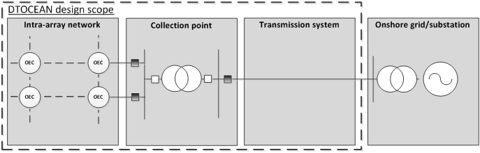
Fig. 6.6 Simplified generic offshore electrical network for OEC arrays

Ultimately, the network design process is defined by the following factors:

• The transmission voltage, capacity and number of transmission cables;
• The number, location and type of offshore collection points;
• The intra-array network topology, i.e. number of OEC devices per string, number of strings, voltage level, and umbilical geometry (for floating devices);
• Optimal cable routing and protection for the transmission system and intra-array cable networks.

These design criteria are constrained by the physical environment, power flow constraints and available components. In order to produce a valid solution within the available design space, the Electrical Sub-System module is driven by the following key concepts.

• Seabed filtering: This filtering process incorporates user-defined exclusion zones and installation equipment compatibility to provide a suitable seabed area for placing electrical components.
• Physical design: The cable routing algorithm designs a route for cables along the seabed.
• Network design: Two network design topologies are considered: radial strings and hub layouts. The network design process utilises a number of heuristics to limit the number of design options; using the relationship between transmission distance, power and voltage to determine acceptable voltage levels for collection point design.
• Power flow analysis: A three-phase steady-state power flow solver is included within the DTOcean tool. This provides AC and DC power flow solution routines.

Using these concepts the Electrical Sub-Systems module selects a toplogy and components in order to produce a local level best solution. This local solution is obtained by calculating and comparing the overall network efficiency (i.e. network losses) and component costs. The realisation of this as structured software is outlined in Fig. 6.7, with cable routing and collection point design functionality shared between the transmission system and intra-array network design.

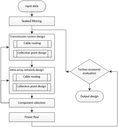
Fig. 6.7 Electrical Sub-Systems model top level view.

6.2.3. Functional specifications

6.2.3.1. Inputs

The required input data to execute the Electrical Sub-Systems modules is given in Fig. 6.8.

Fig. 6.8 Inputs of the Electrical Sub-Systems module.

6.2.3.2. Execution

Once the Electrical Sub-Systems module has been selected and data loaded in the GUI, the user can define a number of options to target the solution in a particular direction. These are defined in Fig. 6.9. These options are also compatible with the DTOCEAN strategy scenario analysis defined in N.N.

Fig. 6.9 User options of the Electrical Sub-Systems module.

6.2.3.3. Outputs

The output data returned by the Electrical Sub-Systems modules is given in Fig. 6.10.

Fig. 6.10 Outputs of the Electrical Sub-Systems module.

6.3. Moorings and Foundations module

6.3.1. Introduction

The main aim of the DTOcean Mooring and Foundation design module is to perform static and quasi-static analysis to inform or develop mooring and foundation solutions that:

• are suitable for a given site, the MRE device (and substation), and expected loading conditions;
• retain the integrity of the electrical umbilical that connects the MRE device to the subsea cable;
• are compatible with the array layout (i.e., prevents clashing of neighbouring devices) and subsea cable layout;
• fulfil requirements and/or constraints determined by the user and/or in terms of reliability and/or environmental concerns; and
• have the lowest capital cost.

6.3.2. Architecture

Dataflow through the module is linear, utilising inputs supplied by the Tool Core but originating from: i) the user (via the graphical user interface (GUI)), ii) the Hydrodynamics and Electrical System Architecture modules (umbilical requirements and subsea infrastructure details) and iii) from the global Tool database. For floating devices the Mooring and Foundation module interacts with the Umbilical sub-module to ensure that the solutions for mooring system and umbilical together are suitable for the site, device and conditions.

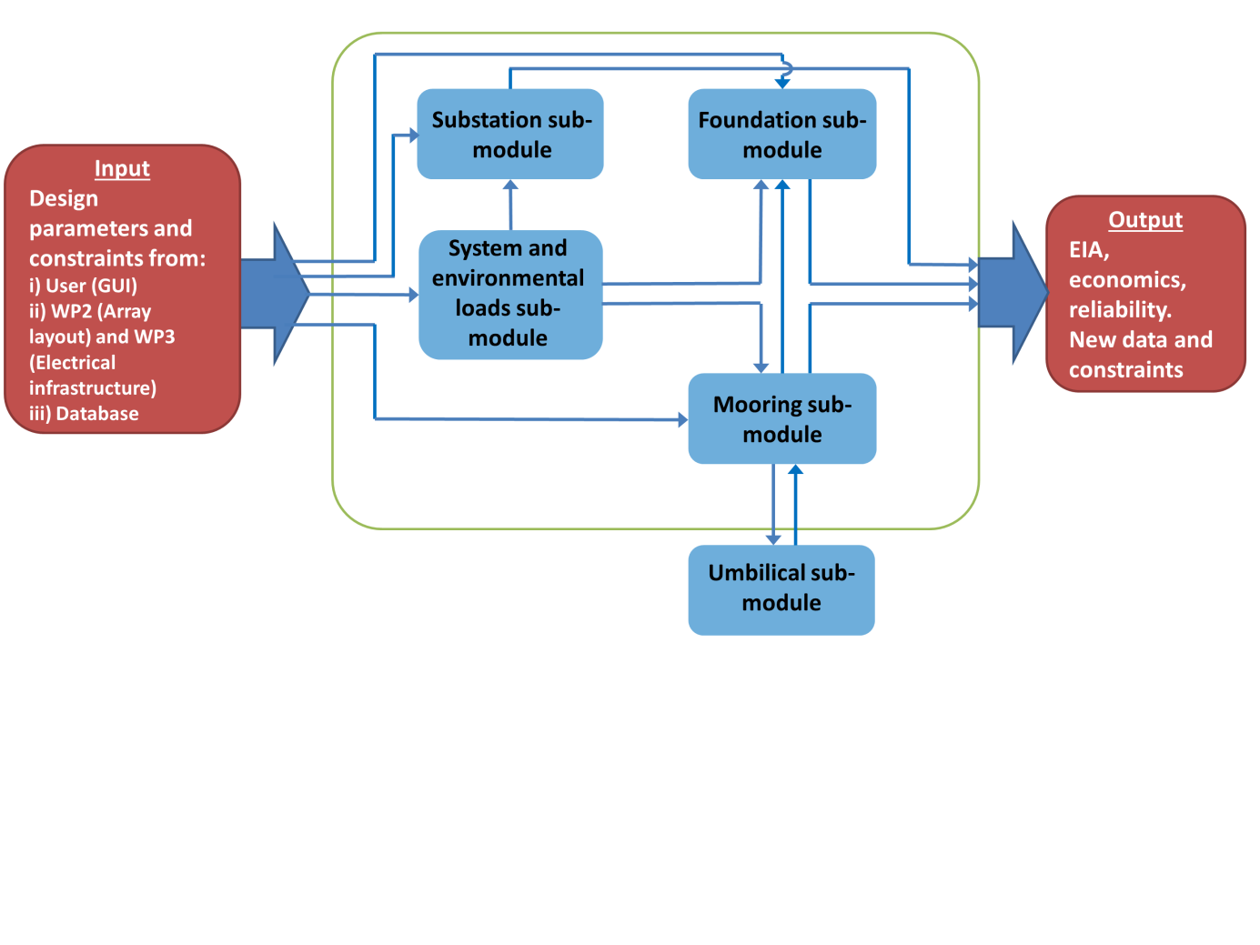
Fig. 6.11 Mooring and foundation module top level view

The Mooring and Foundation module comprises four interlinked sub-modules: the System and environmental loads sub-module, Substation sub-module, Mooring sub-module and Foundation sub-module. In addition the Mooring sub-module communicates with the Umbilical module located outside of the Mooring and Foundation module (with communication occurring via the Tool Core). Fig. 6.11 shows the data flow through the module.

6.3.3. Functional specifications

The use defined inputs are described in the input table below. Certain inputs are listed as optional, where the user chooses not to provide the optional input values then default values will be provided from the database. These inputs will be provided to the tool via the DTOcean graphical user interface.

6.3.3.1. Inputs

The Fig. 6.12 give an overview of the inputs required by the user to run the Mooring and Foundation module. Some of them are compulsory and others are optional.

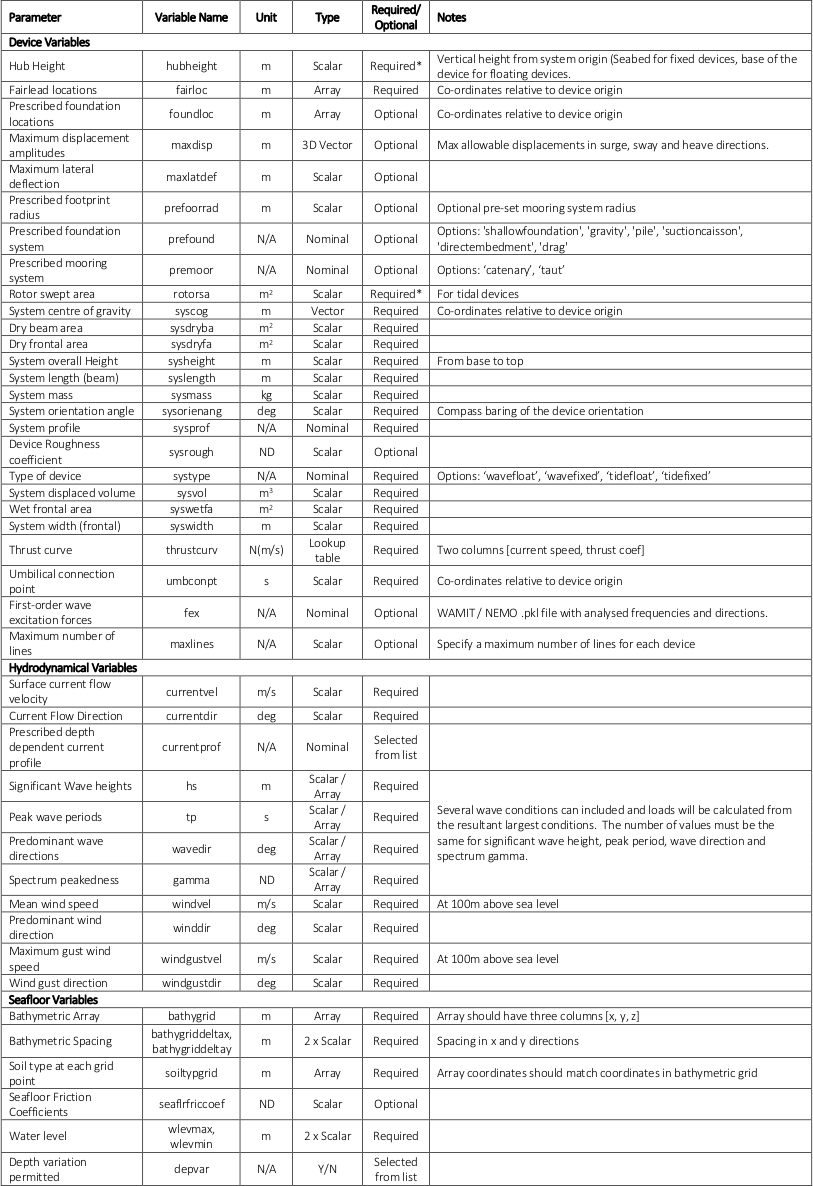
Fig. 6.12 List of inputs for Mooring and foundation module

6.3.3.2. Execution

6.3.3.3. Outputs

The moorings and foundations modules provides the user with output tables detailing the selected mooring, foundation and umbilical design. Several output Tables are created:

• Array level mooring installation table (floating devices only): This details the moorings system design. For each mooring line of each device the type, length and mass are provided and the markers representing all of the individual components are listed (see example in Fig. 6.13).
• Array level foundation installation table: This details the foundation system design. For each anchor or foundation the type, component marker, position, depth, dimensions, installation depth and mass are included. The soil type at the foundation location is listed. For pile type foundation the grout type and volume are provided (see example in Fig. 6.14).
• Array level umbilical installation table: The details the design of the umbilical cable. For each device the component ID and marker number of the umbilical cable is specified. Also specified is the subsea connection point, the depth, length and mass of the cable (see example in Fig. 6.15).
• Array level economics bill of materials: This table lists all of the components used in the mooring, foundation and umbilical system design, the quantity of each and the total cost.
• Array level RAM bill of materials / Array level RAM hierarchy: These tables provides the reliability assessment module with the list of components and their position in the system to enable the reliability calculations to be carried out.

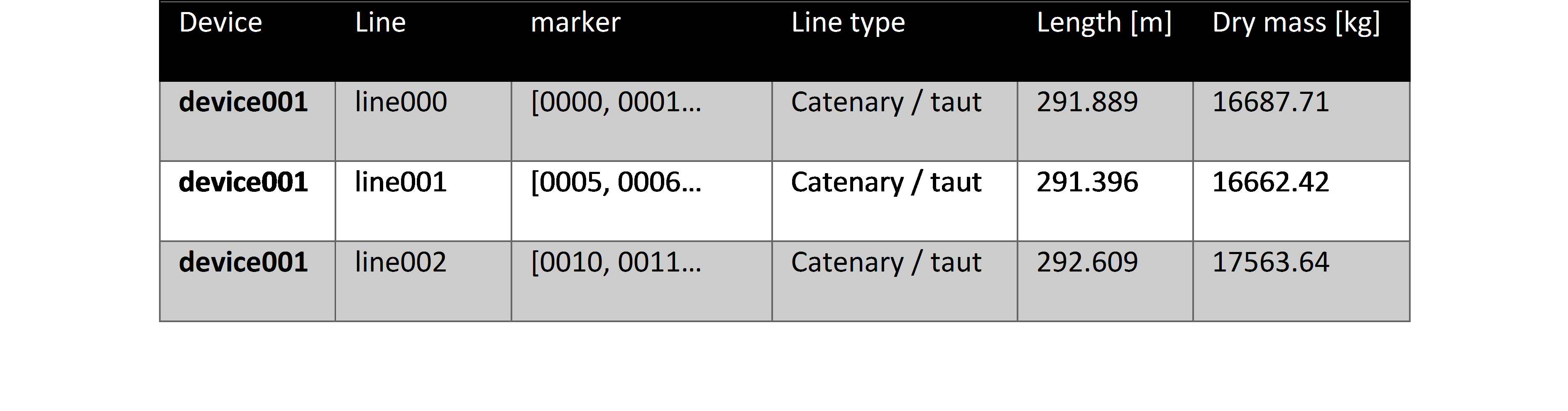
Fig. 6.13 Example output tables : Array Level Mooring Installation Table (floating devices only)

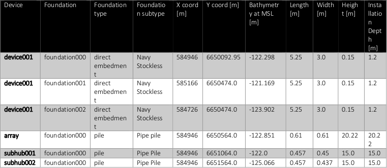
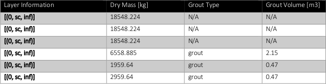
Fig. 6.14 Example of Array level foundation installation table

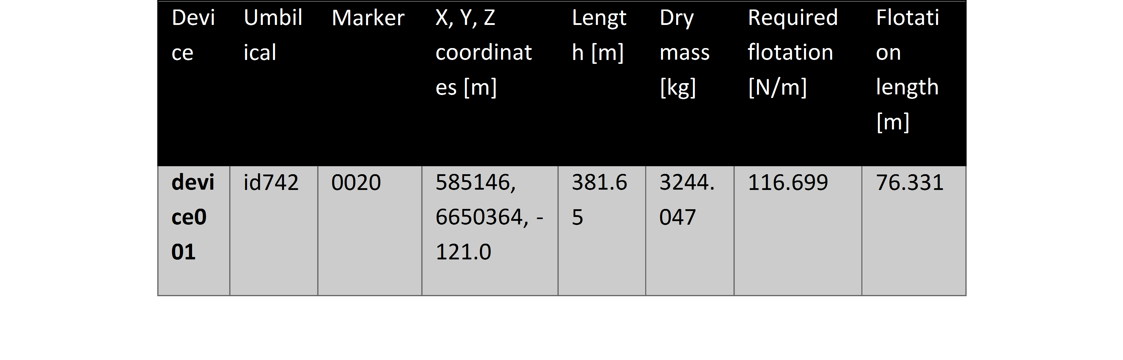
Fig. 6.15 Example of Array Level Umbilical Installation

6.4. Installation module

6.4.1. Introduction

The installation module is seeking to minimize the cost of installation of all components/sub-systems chosen by the upstream modules. It covers the following elements:

• Installation of wave or tidal devices as positioned by the array hydrodynamics module,
• Installation of the electrical infrastructure components as designed by the electrical sub-systems module,
• Installation of the moorings & foundations as arranged by the module.

It should be noted that if the user wishes to use the installation module to assess the installation of only a restricted part of the entire bill of material (comprising devices, moorings & foundations and the electrical infrastructure), then the quantity of the item to be ignored (specified by the user through the GUI of the core module) by the installation module should be set to “zero” by the core. This allows the user to evaluate only the installation of the devices while disregarding the installation of the other components, for example. However, the installation module must always have information about the ocean energy devices to install since it will assume that the starting time for the commissioning will be the latest ending time of all components analysed by the installation module. To facilitate the understanding of the remaining of the user manual for the installation module, here are two definitions of key concepts:

• Logistic operation: refers to a specific task carried out in-land or at sea, e.g the ‘vessel preparation & loading’ or the ‘transportation from port to site’

Logistic phase: is composed of a group of several logistic operations which ultimately forms a marine operation during the installation or O&M stage of a MRE project, e.g ‘installation of the export cable’ or ‘inspection or maintenance of a top-side element on-site’.

6.4.2. Architecture

The installation module comprises complementary features:

• A pre-defined logistic phase sub-module: this is where the logistic operation sequences and vessels & equipment combinations are defined for all logistic phases.
• An installation procedure definition sub-module: it is divided into two functions; one defining the scheduling rules to determine the chronological order of the logistic phases and another function selecting the base installation port.
• An optimization routine: the most inexpensive feasible logistic solution (set of vessel(s), equipment(s) and port) is chosen for each logistic phase.

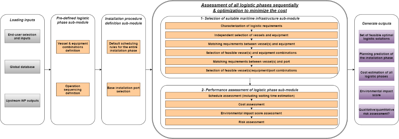
Fig. 6.16 High level flow chart of the installation module

As shown in Fig. 6.16, once the inputs are loaded (first bloc on the left), the installation module runs the two initial sub-modules which serves to define the logistic phases to be considered, their chronological (‘Gantt chart’) relationships and the base installation port. Following this initialization, the assessment of the logistic phases is performed in three steps:

• STEP 1 “selection of suitable maritime infrastructure sub-module”: characterization of the logistic requirements relating the array physical parameters to the characteristics of the maritime infrastructure (ports, vessels and equipment). This step is followed with the matching of the logistic requirements previously determined with the database of vessels, ports and equipment purposely built-in for the DTOcean tool. To avoid unnecessary verification, the selection of the individual vessel(s), port and equipment is constrained by the pre-defined type of vessels and equipment. It can be noted that an advanced user has the opportunity to specify its own set of type of vessel(s) and equipmentby updating existing logistic phase definition Python file or by creating new ones that mimic the existing ones.
• STEP 2 “performance assessment of logistic phase sub-module”: this assessment is three fold:
  • Firstly, an estimation of the schedule of the marine operation is conducted. The mobilization time associated with the availability of the maritime infrastructure (vessels and equipment) is straightforwardly evaluated, based on average values in the vessel database. Similarly, the transportation times are readily computed through the average speed values along with an assessment of the distance from port to site. By combining the total duration of the sea logistic operations and the associated operational limit conditions (e.g max H_s), the expected waiting time associated with the logistic phase can be predicted. This is done through the weather window function which requires the requested starting time and the total sea duration of the logistic phase to return an estimate of the waiting time.
  • Secondly, the cost functions produce estimates of the costs incurred by the utilization of the maritime infrastructure. Both fixed and variable costs are accounted for by making use of relevant economic parameters available in the database of ports, vessels and equipment.
  • Thirdly, a qualitative assessment of the environmental impact associated with the use of the vessel and equipment returns an environmental score for five potential impacts, namely: the risk of chemical pollution, the collision risk, the footprint, the underwater noise and the potential raise of turbidity.
• STEP 3 “optimization routine”: in the logistic module, the objective function is to find the feasible logistic solutions which minimize the total cost (C_lp) of a given logistic phase.

At the end of this process, the outputs of the installation module are sorted and formatted in the a convenient way for post-processing and results visualization purposes. The outputs include a set of optimal feasible logistic solutions along with their schedule, cost and environmental impact assessment.

To cover the scope of the installation of a wave or tidal energy farm, a total of nine logistic phases have been characterized, in terms of:

• List of inputs required to run the logistic phase
• Combinations of vessel(s) & equipment(s) types suitable to carry out the logistic phase
• Feasibility functions pertaining to the selection of individual vessel or equipment that satisfy some requirements such as deck space must be superior to the estimated footprint of one element to be installed
• Feasibility matching to verify the compatibility between vessel(s) and equipment (e.g deck cargo must be superior to the estimated total mass of the equipment and the elements to be installed that are on deck)
• Performance functions depicting the methods (e.g default fixed value or distance multiplied by transit speed) employed to estimate the time and cost per logistic operation.

Any array configuration that can possibly be proposed to the installation module is currently limited to these nine logistic phases characterized. Fig. 6.17 displays the list of the nine logistic phases, split within 3 main categories:

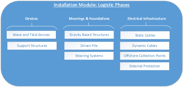
Fig. 6.17 Scope of the logistic phases considered for the installation module

6.4.3. Functional specifications

6.4.3.1. Inputs

The installation module takes a relatively large number of inputs. As a result, the present user manual is only summarizing the nature and content of these required inputs while specifying their origin (end-user entry, upstream module or database). Details of the full list of inputs (parameter description, variable name, unit, format and requirements) can be found in the DTOcean Technical Manual. It should be noted that all input type listed below correspond to a single ‘panda dataframe’ Python format when they are passed to the installation module.

Four types of mandatory inputs originate from the end-user via the GUI:

• “site”; bathymetry and soil type at each point of the lease area
• “metocean”: time-series of wave conditions (H_s and T_p), wind speed and current speed
• “device”: type and main specification of the ocean energy device (e.g dimensions and dry mass). Also includes information about logistic matters such as the assembly and load-out strategies, the transportation method, the estimated time to connect the device at sea and the operational limit conditions during this operation among few others
• “sub_device”: dimensions, dry mass, assembly duration and location of each device sub-system. The device sub-systems were defined generically as follows: A = Main structure, B = Power-Take-Off, C = Control system and D = Support structure (if any)

Three pre-populated databases of mandatory inputs which can be over-written or expanded by the user through the GUI:

• Port database: detailed information about European ports with the following parameter categories:
  • General Information (13 parameters),
  • Port Terminal Specification (17 parameters),
  • Port Cranes, Support, Accessibilities and Certifications (16 parameters),
  • Manufacturing capabilities (8 parameters),
  • Economic Assessment (8 parameters),
  • Contact details (4 parameters),
• Vessel database: detailed information about each vessel types considered in DTOcean with the following parameter categories:
  • General Information (9 parameters),
  • Main Dimensions and Technical Capabilities (18 parameters),
  • Maximum Operational Working Conditions (8 parameters),
  • On-board Equipment Specifications (~34 parameters),
  • Economic Assessment (4 parameters),
• Equipment database: detailed information about each equipment types considered in DTOcean with the following parameter categories (the number of parameters varies from one equipment type to another):
  • Metrology (min. 4 parameters),
  • Performance (min. 2 parameters),
  • Support systems (min. 2 parameters),
  • Economic Assessment (min. 2 parameters),

Other input tables consist of default values which are assumed by the installation module but can be over-written by the user via the GUI:

• Average fixed duration values and OLC values of individual logistic operations (in the table called ‘operations_time_OLC’)
• Vertical penetration rates in all DTOcean soil types for all piling equipment (in the tab ’penet’ of the table ’equipment_perf_rate’),
• Horizontal progress rates in all DTOcean soil types for all cable trenching/laying equipment (in the tab ’laying’ of the table ’equipment_perf_rate’),
• Other generic and diverse costing and time default value assumptions (in the tab ’other’ of the table ’equipment_perf_rate’),
• Safety factors to apply on selected feasibility functions (in the table ‘safety_factors’),
• Default Gantt chart rules (in the table ‘installation order’) for the installation planning.

Finally, there is another type of inputs which can either be generated by upstream modules (i.e “array hydrodynamic module”, “electrical sub-systems module” and “moorings and foundations module”) or specified by the user if the upstream module have not been selected for the run. While the complete detailed list of these inputs can be found in the DTOcean Technical Manual, a summary of their content is provided below.

The inputs expected from the array hydrodynamic module are summarized in Fig. 6.18. It must be noted that this input is compulsory and must contain at least one device since the installation module must always install minimum one device to set the commissioning time for the O&M module and LCOE calculation. Hence, if the user has chosen NOT to select the array hydrodynamic module for the run, it will be necessary to fill out the table below if the installation module is expected to run.

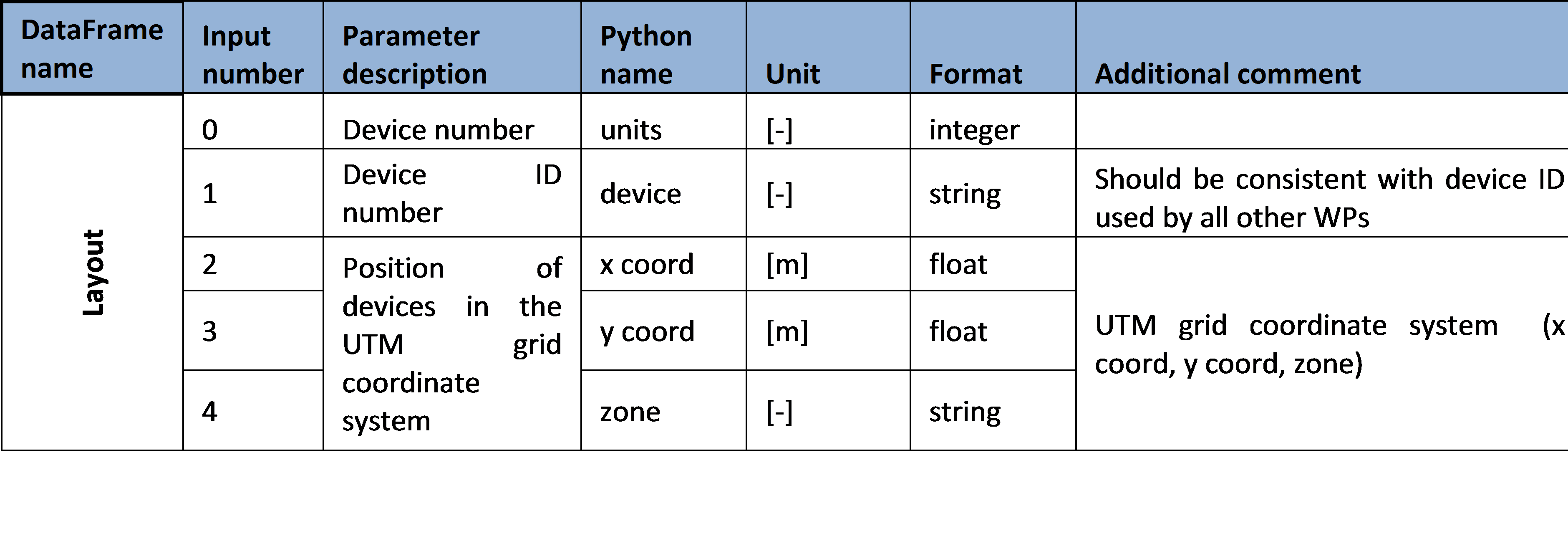
Fig. 6.18 Panda DataFrame containing all required input data generated by the array hydrodynamic module to the installation module

Six panda dataframe Python tables should be passed to the installation module by the electrical sub-system module. Each table refer to a sub-system of an electrical layout of an array of ocean energy devices. Their content can be succinctly described as follows:

• “collection point”: type, coordinates, dry mass, dimensions, interfaces description (upstream and downstream connectors type) and pigtails specifications
• “dynamic cable”: coordinates, dry masses, dimensions, Minimum Bending Radius (MBR). Maximum Breaking Load (MBL), interfaces description (upstream and downstream connectors type) and buoyancy modules specifications
• “static cable”: type, coordinates, dry masses, dimensions, MBR, MBL, interfaces description (upstream and downstream connectors type) and pigtails specifications
• “cable route”: coordinates, soil type, bathymetry, burial depth, split pipe and static cable id
• “external protection”: type and coordinates
• “connectors”: type, dry mass, dimensions and mating/demating forces

Similarly, two panda dataframe Python tables result from the outputs generated by the moorings and foundations module. Below is a summary description (as for all other inputs full details description can be found in the technical manual):

• “foundation”: corresponding device ID, type/subtype, coordinates, dry mass, dimensions, penetration depth, grout type and volume
• “line”: corresponding device ID, type, components list, coordinates, dry mass, length

All the tables originating from upstream module are compulsory but it is possible to have them not populated (i.e empty, except for the table “layout” which must contain at least one device) to signify that there is no need to consider any array-element of one type (e.g collection point or mooring line) for the installation module.

6.4.3.2. Outputs

The list of the outputs from the installation module is given in Fig. 6.19 and Fig. 6.20: it consists of two dictionaries. The first dictionary (see Fig. 6.19) is generated for each logistic phase considered by the installation module (i.e there will be between 1 and 9 of these tables depending on the array elements to be installed). The second output (see Fig. 6.20) contains a summary of the global outputs for the entire installation phase. Both outputs provide information about estimated cost, time and dates of the various operations. Information about the selection of feasible vessel(s), equipment and the base installation port is also given.

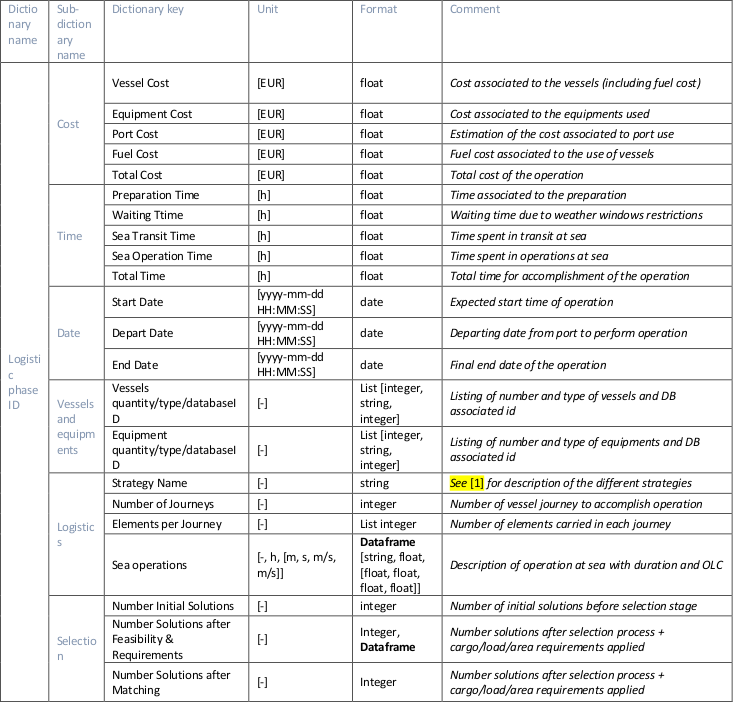
Fig. 6.19 Dictionary output generated for each logistic phase considered by the installation module

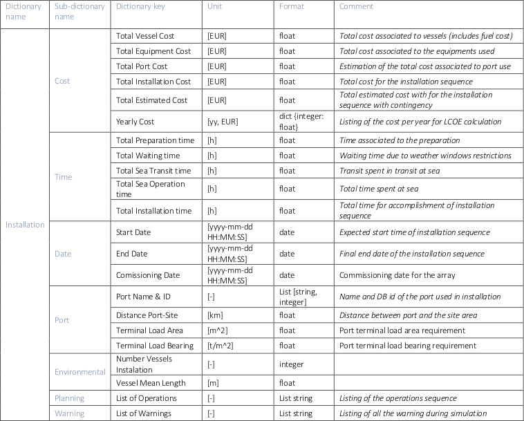
Fig. 6.20 Global dictionary output generated by the installation module

6.5. Operations and maintenance module (OMCO)

6.5.1. Introduction

The purpose of the OMCO module is to simulate the time domain based full life cycle operation and maintenance (O&M) activities of a Marine Renewable Energy (MRE) array. This will consider the costs for the following items:

• OPEX:

  • Vessels (crew transfer, construction, heavy transport, etc.)
  • Equipment (special tools, ROVs, etc.)
  • Personnel (technicians, specialists)
  • Spare parts, materials

• CAPEX:

  • Condition monitoring hardware

The OMCO module simulates all O&M activities of the MRE array over its lifetime in the time domain. Cost related to the O&M activities will be calculated and added to the overall LCOE costs. The OMCO module can be used to understand and optimise the O&M strategy of MRE arrays in the planning phase of a project. The minimisation of the O&M costs will help the decision maker to choose cost-optimal solutions.

Maintenance is defined as the combination of all technical and administrative actions intended to retain an item in, or restore it to, a state in which it can perform its required function. Fig. 6.21 illustrates a common classification of maintenance strategies, which is based on the standard SS-EN 13306.

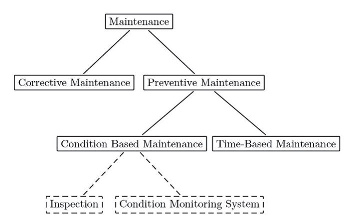
Fig. 6.21 Types of maintenance strategies

The maintenance strategies are considered as defined below:

• Corrective maintenance is due to an unexpected failure and is intended to restore an item/component to a state in which it can perform its required function1.
• Condition-based maintenance is a type of preventive maintenance based on a response to the monitoring information available . It consists of all maintenance strategies involving inspections (noise, visual, etc.) or permanently installed Condition Monitoring Systems (CMS) to decide on the maintenance actions.
• Calendar-based (Time-based) maintenance is a type of preventive maintenance carried out in accordance with established intervals of time or number of units independent of any conditioning investigation2. It is suitable for failures that are age-related and for which the probability distribution of failure can be established based on fixed time intervals.

The O&M costs are known to be an important part of the life cycle OPEX cost of MRE projects. In offshore wind farms, O&M contributes 15-30 % of the total levelised cost of energy (LCOE) . Therefore it is important to develop cost-effective O&M concepts to help MRE projects to be competitive with offshore wind. The optimization of these concepts should address the overall resources required to execute the maintenance activities, which necessarily have to include the logistical support.

To model the individual behaviour of components of MRE array devices, the following items need to be considered:

• Component annual failure rate
• Effect of the failure of the component to other components or devices
• The optimised mixture of the above mentioned strategies to keep the array devices operational
• the requirements of the maintenance processes of all components with respect to time/duration, vessels/equipment, spare parts and personnel

A typical maintenance process is depicted schematically in Fig. 6.22. All maintenance strategies can be simulated with this process plan. The difference in handling the strategies is mostly setting the time parameters to the respective values. For example, for a calendar based or condition based maintenance, the “T_Organisation” will be significantly shorter, since the organisational and preparatory tasks (booking of vessels & equipment, mobilising personnel, ordering of spare parts, etc.) can be done before the scheduled operation starts. Another example is a simple inspection, for which the “T_Logistic” can be set to zero because there is no need for ordering spare parts.

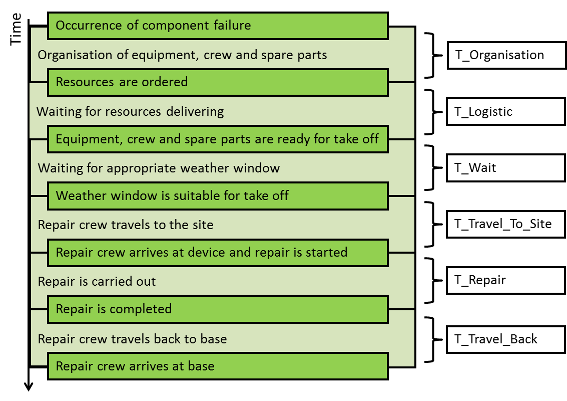
Fig. 6.22 Typical maintenance process

The definition of the calendar based maintenance is simply done by setting the interval (e. g. “annual”, “semi-Annual”, etc.). The condition based maintenance required the definition of a “state of health” (SOH) threshold, below which maintenance is mandatory for the component. For this, it is assumed that at the installation / commissioning of a MRE device or after repair / replacement activities, the SOH of a component will be 100%. A linear interpolation simulates the SOH of the considered component. The SOH limit in % that triggers the condition based maintenance is a parameter of the OMCO module and will be set by the user. The slope of the SOH degradation curve is also defined by the user.

Fig. 6.23 Handling of automated inspection in case of condition-based maintenance

In the time domain simulation the occurrence of failures has to be estimated over the lifetime of the device. To translate the statistical based failure rates back to the time domain, a Binomial or Poisson process is used. A Poisson process is a stochastic process that counts the number of events and the time points at which these events occur in a given time interval. The time between each pair of consecutive events has an exponential distribution with parameter λ (intensity) and each of them inter-arrival times is assumed to be independent of other inter-arrival times. Fig. 6.24 depicts an example of a Poisson process.

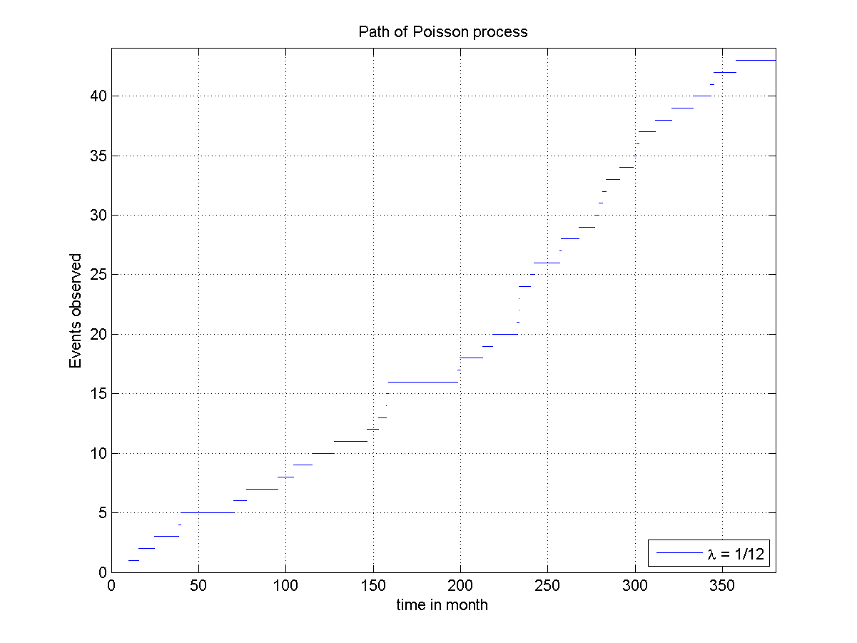
Fig. 6.24 Paths of Poisson process for a 30 year period and a number of 44 events

For time domain simulation purpose, a maintenance plan will be generated for each relevant component as defined by the user. Everything inside the array will be handled as a component, i. e. a component can be:

• an infrastructure item, e. g. the export cable, the sub-station(s), subsea connectors, switch gear, cable sections in the internal array grid, etc.
• an entire device (if no deeper level of detail is required)
• components of a device (level of detail will be restricted to the Equimar definition with the four major sub-systems: hydrodynamic converter, PTO, reaction and controller)

For each component, a maintenance plan will be generated. Fig. 6.25 shows an example. Each maintenance type has its own colour code:.

Fig. 6.25 The Schematic overview of a maintenance plan

6.5.2. Architecture

The functional structure of the OMCO module is shown in Fig. 6.26. The module at hand here is a “computational package”. This means that all input for the module comes via the core module as represented by the grey “User Definitions” block. Such user definitions need to be stored in the global data base and will be read out by the core module and then passed to the OMCO. Any output calculated in the OMCO will be passed back to the core (“Results” block).

The module uses embedded code, i. e. it reads the array configuration and the failure rates for all components from the “Reliability Assessment Module” (RAM), which is an external module providing information about the array layout and the failure probability (as annual failure rates).

For each of the components in scope, an individual maintenance plans will be initialised. In a first request, the logistic functions will be called to retrieve the availability of vessels and equipment (V&E). If required, the maintenance plans will be updated. In a second step, the optimisation loop(s) will be performed

In the “Maintenance Strategies” block, the array structure will be translated in several module objects. With this objects, each representing one component, all relevant elements will be generated as class instances in the executable code.

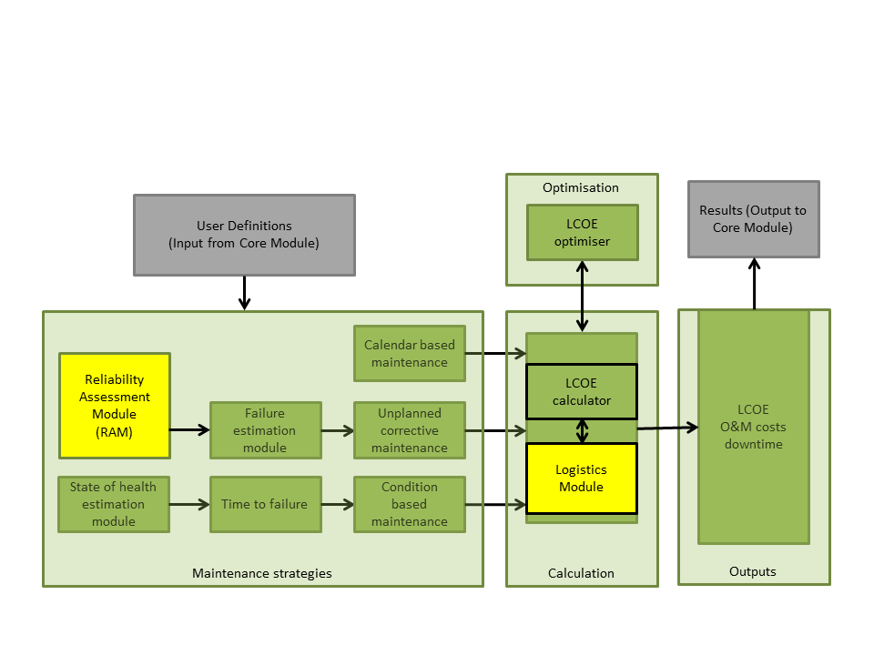
Fig. 6.26 OMCO module functional structure

Once all the classes are implemented, the optimisation loop (“Calculation” block) runs and sequentially calls several logistic functions to execute the O&M cost calculation. The loop runs until there is a minimum LCOE is achieved.

6.5.3. Functional specifications

6.5.3.1. Inputs

The following table contains the description of the parameters which are common for all components in the array

The following tables contain the description of the parameters for definition of the electrical components in the array’s balance of plant. There are four parameter categories to be considered:

Category 1: “Component”

Category 2: “FailureModes”

Category 3: “RepairActions”

Category 4: “Inspections”

The following tables contain the description of the parameters for definition of the devices in the array and, if applicable, their individual components. There are four parameter categories to be considered (there structure is very similar to the one as for the electrical components. For better readability, the deviating parts are highlighted in light blue):

Category 1: “Component”

Category 2: “FailureModes”

Category 3: “RepairActions”

Category 4: “Inspections”

Notes:

1. allowed values are “Substation”, “Export Cable”, “Subhub”
2. Definition of FM IDs

3. CAPEX costs for condition monitoring hardware: it is assumed that the hardware is not installed in the component/device during production. If the device is purchased with an already installed condition monitoring hardware, set value(s) to “0”;
4. allowed values for component type
   • Hydrodynamic
   • Pto
   • Control
   • Support structure
   • Mooring line
   • Foundation
   • Dynamic cable
   • Array elec sub-System

6.5.3.2. Execution

After adding the “Operation and Maintenance” module to the list of active modules and of the proper setting up of the required data base parameters (as described in the section above), the only thing remaining is the selection of the desired maintenance strategy (or all possible combinations of multiple strategies) by the user. This can be done by using checkboxes like in the example given below.

Fig. 6.27 Checkbox for the selection of different combinations of maintenance strategies

When all setup is done, the “Operation and Maintenance” module can be executed in the frame of an optimisation run of the core program.

6.5.3.3. Outputs

After execution of the “Operation and Maintenance” module, the following output parameters will be passed to the user via the core module:

The table below gives some examples for values resulting from a test run with two devices defined in an array.