8. DTOcean Themes
8.1. Economics Module (EM)
8.1.1. Requirements
8.1.1.1. User Requirements
The ‘economic assessment’ module takes the array configuration determined by the design modules previously described and estimates the LCOE for the project. The LCOE is the indicator used for benchmarking different possible solutions, and the global optimization routine objective is to minimize it.
Within each design module there are economic functions that calculate the lifetime costs of the corresponding subsystem. These will be used as input for the LCOE calculation.
The ‘economic assessment’ module is composed of a set of functions that are used to calculate the LCOE, which can be called separately or as a whole. It requires information from all the other modules, as well as user inputs.
8.1.1.2. Software Design Requirements
For the total LCOE calculation, a list of components used for the project is to be provided from the other com- putation design modules, with the required quantities and the related cost, which will have been calculated within each of these modules or provided by the database or the end-user.
The current ‘economic assessment’ module includes four separate functions, although “df_lcoe” is the integration of the other three:
- item_total_cost
- present_value
- simple_lcoe
- df_lcoe
The functions and their interactions with the inputs are presented in a diagrammatic form in Fig. 8.13. A more detailed explanation of each component can be found further in this document.
The first three functions can take single or multiple values as inputs, while the last one assumes that the inputs are in the format of pandas tables, with specific columns.
For the df_lcoe function, two tables are expected as inputs:
- Bill of materials table, including the following columns:
- item: identifier column, not used in the function
- quantity: number of units of item
- unitary_cost: cost per unit of the item. It assumes that it matches the units of the quantity
- project_year: year relative to the start of the project when the cost occurs (from year 0 to the end of the project)
- Energy output table, including the following columns:
- project_year: year relative to the start of the project when the cost occurs (from year 0 to the end of the project)
- energy: final annual energy output. This value accounts for the hydrodynamic interaction, transmis- sion losses and downtime losses
The other input of the df_lcoe function is the discount rate, which is assumed to remain constant during the lifetime of the project, and is a single float value from 0. to 1. to represent the discount rate percentage.
8.1.2. Architecture
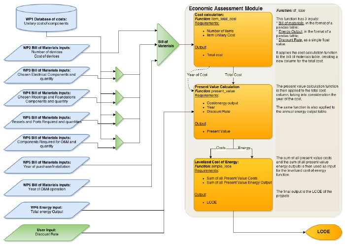
Fig. 8.13 Detailed flowchart of the economic assessment module
The function item_total_cost takes the information of quantity and unitary cost and calculates the total cost within the context of the array in analysis. At this stage it is a simple multiplication, but it could be expanded to account for scaling factors or bulk discounts.
Furthermore, the function assumes that all cost data is presented in the right units to match the quantities, and that the currency is the same. Further functions dealing with units and currency conversion could be developed.
The cost values can, at most, be grouped by year, as the present value function will have to be applied before the LCOE calculation. However, it can be interesting for the user and for the other modules to have the total cost values detailed by activity (or by design module) or even at an item level.
The function present_value transforms any future value into a present value assuming a specific discount rate. The present value function is applied to costs and energy output, using the discount rate set by the user. To calculate the present value of the costs, this function assumes that the total cost has already been calculated using the previous function. If the year-on-year costs are equal, the present value can be calculated for lump sums, instead of on an item by item basis.
The function simple_lcoe uses the sum of the present values, as in the formula below, calculated with the previous function as inputs: sum of all costs and sum of all energy outputs.
The function df_lcoe takes the preformatted inputs in the format of pandas DataFrame tables (bill of materials, energy output), as described in the previous section and applies the previous functions.
For the BoM table, the function creates a new column (‘cost’) for present value of the total cost, by applying first the item_total_cost function, and then the present_value one. It then sums all the cost calculated, which will be the first input for the simple_lcoe function.
For the energy output table, the function creates a new column (‘discounted_energy’) by applying the present_value function. Like in the previous table, it then sums all the calculated energy outputs. This sum will be the second input for the simple_lcoe function.
The output of this function is the LCOE, expressed in €/MWh.
Intermediate or other functions could be developed to evaluate how the LCOE changes during the project lifetime as an extension to the base functionality.
8.1.3. Functional Specification
The cost of the OEC devices can be provided by the user as an optional input. As with the other costs assumed in the software, these are expected to be given in Euro currency.
The discount rate is also to be provided by the user, as it is dependent on the investor’s valuation of risk and investment opportunities. Typical values of discount rate for marine energy projects range between 8-15% (Allan et al., 2011; Andrés et al., 2014; Carbon Trust, 2011, 2006; Ernst & Young and Black & Veatch, 2010; SQWenergy, 2010) but in LCOE evolution analysis is typical to use values between 10% and 12% (Carbon Trust, 2006, p. 200; OES, 2015; SI-OCEAN, 2013). More information on the discount rate can be found elsewhere (DTOcean, 2015j).
The dates at which costs are incurred are also required as an input and will be an output from the Installation and O&M modules. Alternatively, for capital expenditures, it could be assumed that all costs occur in year zero.
The final input required from the other design modules is the annual energy output. To the calculation of the LCOE only the final energy output is needed, which to be provided by the operations and maintenance module after the downtime has been assessed. However, the input of the LCOE function could also be the unconstrained energy, but it should be noted that then the LCOE will be underestimated. There is value is calculating this overoptimistic LCOE, as it provides a metric on the impact of downtime and other losses calculated by the software.
The main output of the ‘economic assessment module’ is the LCOE, presented in terms of €/MWh. Other outputs can be produced from the building blocks of the LCOE function, such as total lifetime costs (presented in €) and the total expected electricity production (expressed in MWh).
8.1.3.1. Inputs
The Economics module requires inputs from other modules and from the user. The inputs from other modules can always be overwritten by the user.
The Bill of Materials is generated by the core from the outputs of the other design modules. It is formatted as a pandas tables, with the following fields:
- item: identifier column, not used in the function
- quantity: number of units of item
- unitary_cost: cost per unit of the item. It assumes that it matches the units of the quantity
- project_year: year relative to the start of the project when the cost occurs (from year 0 to the end of the project)
The second set of inputs generated by the tool relates to the energy production. It also formatted as a pandas table, with the following columns
- project_year: year relative to the start of the project when the cost occurs (from year 0 to the end of the project)
- energy: final annual energy output. This value accounts for the hydrodynamic interaction, transmission losses and downtime losses
The project_capacity input, referring to project capacity in MW, is an output from the Array Hydrodynamic module, by using the number of devices output and the user input on device rating.
The inputs a_energy_wo_elosses and a_energy_wo_availability are outputs from the the Array hydrodynamic and Electrical sub-systems modules, respectively. The input a_energy_wo_elosses indicates the average annual unconstrained energy production, before electrical losses; while a_energy_wo_availability indicates the average annual energy production accounting for electrical losses, but without accounting for availability.
From the user, the following inputs are required:
- project_lifetime: duration of the project in number of years
- discount_rate: discount rate for the project in analysis. The discount rate is dependent on the investor’s valuation of risk and other investment opportunities.
8.1.3.2. Outputs
The main output of the economics theme module is the levelized cost of energy (LCOE) of the project, expressed in €/MW. The building blocks of the LCOE calculation, CAPEX, OPEX and Annual Energy Production, are also outputs of the module
This allows for the representation of the contribution of CAPEX and OPEX to the LCOE, the contribution of each sub-system/module, or the evaluation per device.
8.2. Reliability Assessment Module
In this section the requirements, architecture and functional specification of the Reliability Assessment sub-module (RAM) are summarised.
8.2.1. Requirements
In this section the requirements, architecture and functional specification of the Reliability Assessment sub-module (RAM) are summarised.
8.2.1.1. User Requirements
Reliability assessment is one of the three main thematic assessment requirements of the DTOcean software. At first, the design modules (Electrical Sub-Systems and Moorings and Foundations) will produce a solution which is unconstrained in terms of environmental impact and reliability but focused on achieving the lowest possible capital cost. Installation and O&M scheduling will take place in the respective module by making use of the logistic functions. The role of the RAM sub-module will be to conduct reliability calculations for i) the user and ii) to inform operations and maintenance requirements of the O&M module.
The purpose of the RAM is to:
- Generate a system-level reliability equation based on the inter-relationships between sub-systems and components (as specified by the Electrical Sub-Systems and Moorings and Foundations component hierarchies and by the user)
- Provide the user with the opportunity to populate sub-systems not covered by the DTOcean software (e.g. power take-off, control system) using a GUI-based Reliability Block Diagram
- Consider multiple failure severity classes (i.e. critical and non-critical) to inform repair action maintenance scheduling. This will represent a simplified approach to Failure Mode and Effects Analysis (FMEA)
- Carry out normal, optimistic and pessimistic reliability calculations to determine estimation sensitivity to failure rate variability and quality analysis
- Provide the time-dependent failure estimation model (in the O&M module) with the Time to failure (TTF) of components within the system
It will produce:
- A pass/fail Boolean compared to user-defined threshold
- Distribution of system reliability (%) from mission start to mission end (\(0 \le t \le T\)).
- Mean time to failure (MTTF) of the system, sub-systems and components presented to the user in a tree format
- Risk Priority Numbers (RPNs)
8.2.1.2. Software Design Requirements
The RAM has been developed to calculate reliability metrics for each component or sub-system provided by the database and/or user. It is a separate module which is fed input specified by the user, database and design modules (via the core for the global design) and provides reliability statistics to the O&M module and user GUI (again via the Core, see Fig. 8.14).
If a proposed design solution is not feasible in terms of reliability (i.e. it does not match the threshold set by the user) after the initial run of the software, an alternative solution will be sought by initializing a subsequent run of the software. For example, if the reliability of a proposed mooring system is unacceptable then a constraint could be fed back to the Moorings and Foundations module. Therefore, only components with a reliability level above a certain threshold (based on the required level of system reliability set by the user) would be available for selection when the Moorings and Foundations module is re-run.
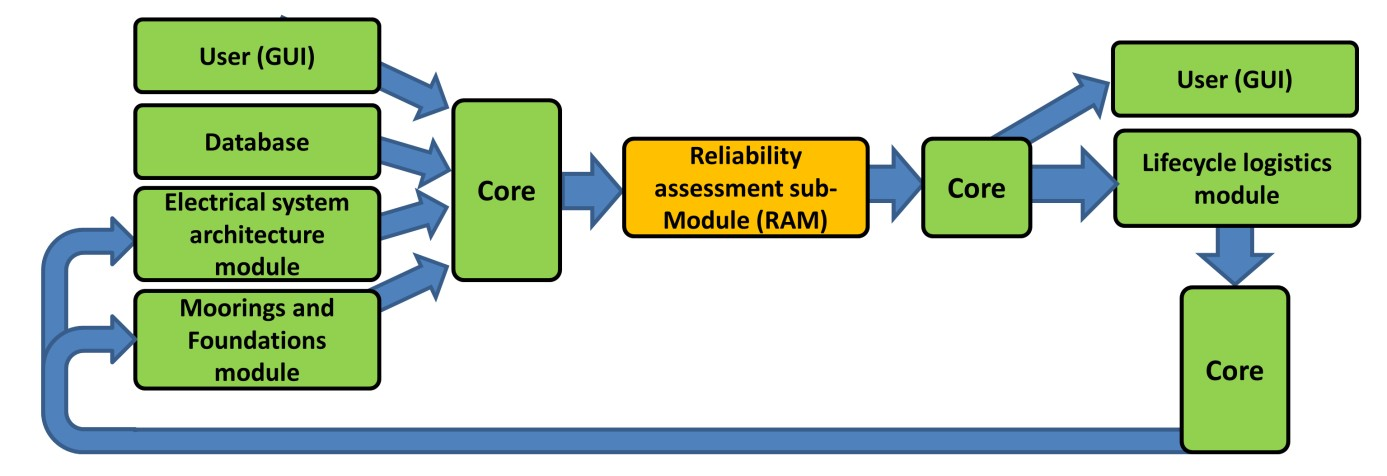
Fig. 8.14 Interaction of the Reliability Assessment sub-module with the other components in the software
The 3rd party Python packages used by the RAM are as follows:
- matplotlib
- numpy
- pandas
Starting with the lowest analysed level (component level), the algorithms used to calculated reliability at a specified time (i.e. mission time) are introduced in the following subsections.
8.2.1.3. Component reliability
Assuming an exponential distribution of failures component reliability is calculated as:
where \(\lambda\) is the component failure rate.
8.2.1.4. Reliability of higher system levels
For higher system levels (sub-system, device, device cluster, string and array) reliability at mission time is calculated in several ways depending on the relationships between adjacent system elements, as defined by the User, Electrical System Architecture and Mooring and Foundation system hierarchies.
For series relationships comprising n elements:
For parallel relationships comprising n elements:
For the special case of ‘m of n’ relationships, such as multiple mooring lines:
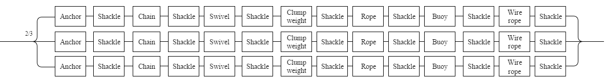
Fig. 8.15 Example mooring system comprising 3 lines
8.2.1.5. Component MTTF
Component MTTF values are calculated as the reciprocal of the specified failure rate:
8.2.1.6. MTTF of higher system levels
Similarly to the reliability metric described above for higher system levels (sub-system, device, device cluster, string and array) the method of calculating MTTF is dependent on if adjacent elements are in series, parallel or belong to an ‘m of n’ system.
For series relationships:
For parallel relationships binomial expansion of terms is required:
Finally for ‘m of n’ relationships:
8.2.2. Architecture
8.2.2.1. Overview
The RAM comprises two Python modules (Fig. 8.16). RAM_Main.py acts as an interface between the user and the module and also calls the functions within the RAM. RAM_Core.py comprises the classes and functions required to carry out statistical analysis of the system. As can be seen from Figure 7.5 with RAM_Core.py there is interaction between the functions within the Syshier class. The use of result sets by the O&M module is discussed in later sections.

Fig. 8.16 Interaction between the various classes and methods of the Reliability Assessment sub-module
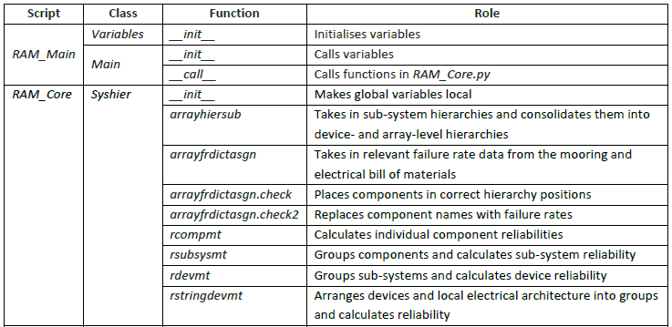
Fig. 8.17 Summary of internal RAM processes
SYSTEM HIERARCHY
In order to generate the reliability equations at each system level, component hierarchies defined by the Electrical Sub-Systems and Moorings and Foundations modules (which specify the inter-relationships between components and sub-systems) are used. In addition, any user-specified sub-systems are included at this stage. At the top level of the hierarchy each device will be identified by its DeviceID number. To implement this structure in Python, nested lists have been used, for example the table below shows a simple device and substation foundation example.
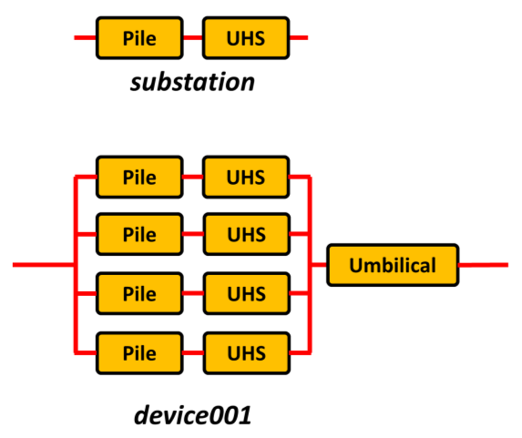
Fig. 8.18 Example hierarchy configuration from the Moorings and Foundations module
Assuming that the same components are used for each of the four devices in the example array, the Moorings and Foundations hierarchy in Python would appear as:
{'array': {'Substation foundation': ['pile', 'UHS']},
'device001': {'Foundation': [['pile', 'UHS'], ['pile', 'UHS'], ['pile', 'UHS'], ['pile', 'UHS']],
'Umbilical': ['submarine umbilical cable 6/10kV']},
'device002': {'Foundation': [['pile', 'UHS'], ['pile', 'UHS'], ['pile', 'UHS'], ['pile', 'UHS']],
'Umbilical': ['submarine umbilical cable 6/10kV']},
'device003': {'Foundation': [['pile', 'UHS'], ['pile', 'UHS'], ['pile', 'UHS'], ['pile', 'UHS']],
'Umbilical': ['submarine umbilical cable 6/10kV']},
'device004': {'Foundation': [['pile', 'UHS'], ['pile', 'UHS'], ['pile', 'UHS'], ['pile', 'UHS']],
'Umbilical': ['submarine umbilical cable 6/10kV']}}
It is possible to identify parallel and series relationships from this list since the component names are separated: series components are separated by a comma whereas parallel relationships are indicated by square brackets. By default mooring systems are treated as ‘m of n’ systems (where \(m=n-1\)) to represent an Accident Limit State scenario (Det Norske Veritas, 2013a).
FAILURE RATE DATA
Reliability calculations performed within the RAM are based on the assumption that failures follow an exponential distribution and hence that the hazard rate is constant with time. Being open-source software, other distributions could be included in the future to incorporate the two other main life stages (burn-in and wear-out).
Based on the component names identified in the hierarchy list, failure rates from the database will then be accessed. Failure data for certain components may be sparse. A review8 of mooring component failures of production and non-production platforms and vessels illustrates this point. Most, if not all of these failures can be classified as critical: although redundancy is usually taken into account while designing these types of mooring systems, immediate intervention would be required to regain system integrity. Assumptions will have to be made if data is not available for all components (i.e. using the failure rates of similar components or sub-systems).
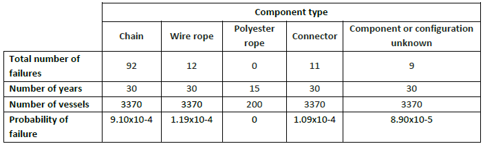
Fig. 8.19 Reported non-production mooring failures 1981-2009 and estimated probability of failure (based on a 30 year interval)
FAILURE TYPES
Clearly not all failures will result in system downtime and some may be sufficiently minor to warrant delaying replacement until the next maintenance interval. The OREDA Offshore Reliability Data Handbook (OREDA, 2009) which is widely used in the offshore oil and gas industry defines three failure severity levels:
- Critical failure – a failure which causes immediate and complete loss of an equipment unit’s capability of providing its output
- Degraded failure – a failure which is not critical but prevents the unit from providing its output within specifications. Such a failure would usually, but not necessarily, be gradual or partial, and may develop into a critical failure in time
- Incipient failure – a failure which does not immediately cause loss of an equipment unit’s capacity of providing its output, but which, if not attend to, could result in a critical or degraded failure in the near future
Within the RAM, two failure mode categories are used to distinguish between the different consequences of failure: i) critical and ii) non-critical (encompassing failures described by the ‘degraded’ and ‘incipient’ definitions above). The corresponding parameters are failratecrit and failratenoncrit.
Within the O&M module, O&M scheduling will be based on the probability of failure, failure mode and required repair action. Two runs of the RAM will be conducted using the different failure rates associated with critical or non-critical severity levels. This is effectively a simplified version of FMEA, but assumes that all failures are independent (i.e. there are no cascade failures).
Furthermore, it is unlikely that failure data will be available for all severity classes. Therefore, by default RAM calculations are based on failure rates associated with the highest available severity levels, with subsequent runs utilising lower severity level values (where available).
CONFIDENCE LEVELS
Failure rates are often specified as single values, which usually correspond to a calculated mean of many samples, possibly from multiple installations. A single value does not provide any information on the variability of component reliability over multiple installations (or the presence of outlying failures) which could have a significant impact on the overall MTTF of the system and associated system downtime and costs. Uncertainty levels provide a measure of confidence of the baseline failure rate. If upper and lower uncertainty levels are specified, the RAM functions will be called several times using lower, mean and upper level failure rates. Therefore failratecrit and failratenoncrit are 1 x 3 vectors for each component. Three estimation scenarios are hence provided, which are ‘optimistic’, ‘normal’ and ‘pessimistic’ from which the sensitivity of lifecycle costs over the duration of the project can be analysed.
In addition to performing calculations with lower, mean and upper uncertainty level failure rates, these values will be reported to the user to enable the quality of the estimate if the sample population (which the failure rate is based upon).
8.2.2.2. Result sets and the O&M module
Considering the two severity levels (ULS, ALS) and three failure rate confidence levels (upper, mean andlower) introduced in above, six result sets are generated by the RAM. It is highly unlikely, given the current state of the MRE sector, that failure rate data will be available for all six factors for all components. To cater for the situation where data is limited for some components, runs of the RAM for lower and upper uncertainty levels and non-critical failures will use mean, critical failure rates for these components. This enables full system analysis to be conducted even if a complete set of data is not available. The time domain calculations which take place within the O&M module are computationally demanding in terms of the time required to simulate failure events for all components in a system. To avoid the need to analyse all of the six result sets from the RAM, the O&M module will only focus on a ‘best’ and ‘worst’ case scenario related to highest and lowest calculated TTFs.
The base design of the module does not contain an optimisation function; it simply calculates reliability metrics based on the provided information. An extension could be provided so that if the calculated MTTF of the system does not meet the user-specified target, the RAM will try to identify which part of the system can be improved in terms of reliability (i.e. which sub-system has the lowest overall reliability) and request that changes are made by the corresponding module (Moorings and Foundations or Electrical Sub-Systems). Once changes have been made (i.e. replacing a component with a more reliable, but perhaps more costly equivalent) the RAM will be rerun.
8.2.3. Functional specification
8.2.3.1. Inputs
The input parameters required by the RAM, their format and source (or destination) are provided below:

8.2.3.2. Outputs
The output parameters provided to the O&M, Electrical Sub-Systems and Moorings and Foundations modules and the user are described here:

Within the following subsections several of the inputs and outputs are explained in more detail. The user-defined hierarchy and BoM will both be empty by default (i.e. and hence all device sub-systems apart from the Moorings and Foundations and Electrical Sub-Systems are assumed to never fail). If the user wishes to populate the system with blocks to represent devices or devices comprising multiple sub-systems (i.e. for the power take-off system, structure etc.) this is possible via a reliability block diagram. The minimum required data for the RAM to function is a mean failure rate (by default this is assumed to represent a critical failure) for each device or sub-system.
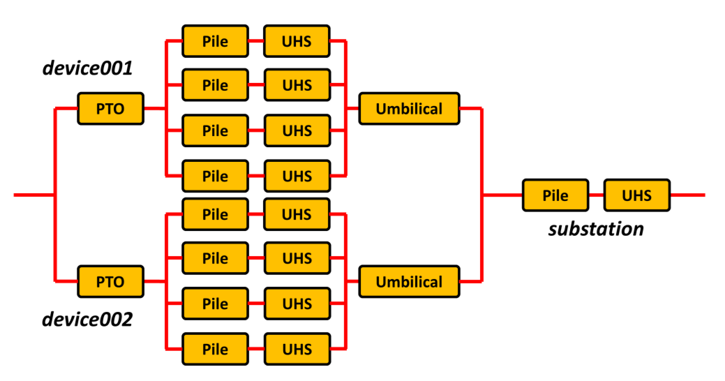
Fig. 8.20 Example parallel configuration including Moorings and Foundations elements and user specified power take off (PTO) sub-systems for two devices. For brevity inter-array cabling and the export cable are not shown
For the example shown in Fig. 8.20 the hierarchy and bill of materials for the user-defined PTO systems are shown below:
Hierarchy
{'device001': {'Power take off system': ['generator']},
'device002': {'Power take off system': ['generator']}}

Bill of materials
{'device001': {'quantity': Counter({'generator': 1})},
'device002': {'quantity': Counter({'generator': 1})}}
In this way the user can specify additional elements down to component level. For example if the user wished to include a gearbox the hierarchy and bill of materials would become:
Hierarchy
{'device001': {'Power take off system': ['generator', ‘gearbox’]},
'device002': {'Power take off system': ['generator', ‘gearbox’]}}

Bill of materials
{'device001': {'quantity': Counter({'generator': 1, 'gearbox': 1})},
'device002': {'quantity': Counter({'generator': 1,'gearbox': 1})}}
The main outputs of the RAM are component MTTFs (which are used by the O&M module), information for the user and results stored in a log file. Reliability information is presented to the user via a tree structure. The tree provides a breakdown of the calculated system reliability into sub-system and component levels, thereby allowing the user to explore the system (i.e. locate components with low reliability). The following information is provided in the tree structure:
- System, subsystem or component name
- MTTF
- Risk priority numbers
Risk priority numbers are calculated within the RAM based on the frequency of failure and severity level of each component. Using the approach suggested in (National Renewable Energy Laboratory, 2014) failure frequency bands are defined by estimated probability of failure ranges (Fig. 8.21). RPNs increase with failure frequency and severity level and can be colour-coded (Fig. 8.22).
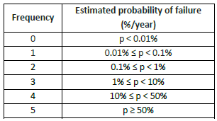
Fig. 8.21 Failure frequencies for several probability of failure ranges (from (National Renewable Energy Laboratory, 2014))
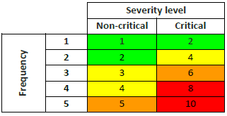
Fig. 8.22 Risk Priority Number matrix with possible colour coding scheme (adapted from (National Renewable Energy Laboratory, 2014))
In order for the user to be able to identify high-risk components and sub-systems which may require unplanned corrective maintenance, the calculated RPNs and time-varying system reliability are also presented here.
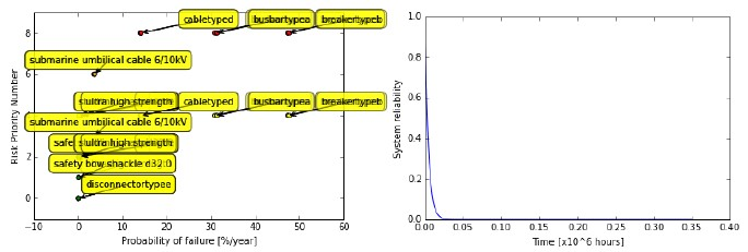
Fig. 8.23 Example (left) RPN and (right) system reliability plots
8.3. Environmental Impact Assessment Module
8.3.1. Introduction
The purpose of the Environmental Impact Assessment (EIA) is to assess the environmental impacts generated by the various technological choices taken by the design modules when optimising an array of OEC devices.
The EIA consists of a set of functions that are able to qualify and quantify the potential pressures generated by the array of wave or tidal devices on the marine environment. It uses two types of inputs. Some data will have to be provided by the user; other data will come directly from the other modules (e.g. Hydrodynamics, Electrical architecture, Moorings and Foundations etc.).
The EIA is based on several scoring principles which are detailed in this chapter of the Technical Manual. In summary, the use of the environmental functions allows the EIA to generate numerical values that will be converted into environmental scores (EIS - Environmental Impact Score). The conversion from the function’ scores to the environmental scores are made through calibration matrices. Each function is associated with one calibration matrix (or several depending on the complexity of the function) in order to qualify the initial pressure score. Calibration matrices are based on literature data or empirical data together with a weighting protocol which is implemented in the EIA logic to better qualify the environmental impacts.
The scoring allocation system developed within the DTOcean framework is generic for each environmental function and based in three consecutive main steps. The first step consists of qualifying and quantifying the ‘pressure’ generated by all components introduced in the the water. This could be, for example, the generation of underwater noise or a footprint from the device foundations. The second step is to define if there are some ‘receptors’ or not in the area that is potentially affected by the pressures generated in the first step. Receptors can be mammals, birds or habitats. Within the receptors, some distinctions are made depending on their sensitivities to the pressures. Some receptors are also identified as ‘very sensitive’ e.g. regulatory protected species. The last step consists of a refinement of the receptor’s qualification with the definition of their seasonal distribution (occurrence or absence on site during the year).
The EIA should inform the user about the ‘environmental impact’, including adverse but also potentially positive impact, of the technological choices and options made during each individual design module, as well as their combined effect.
Recommendations based on the pressure and the receptor’s score are provided to the user to help improve the environmental impact of the proposed array using more environmental friendly solutions.
8.3.2. Global Concept of the Module
Environmental risk assessment is a process that estimates the likelihood and consequence of adverse (or positive) environmental impacts (United States Environmental Protection Agency, 2015). In that regard, conceptual model development is critical to assessing the environmental risk. The approach used here is based on the concept of environmental effects generated by ‘stressors’ and the related exposure of ‘receptors’ to these effects. A stressor is any physical, chemical, or biological entity that can induce an adverse response. Stressors may adversely affect specific natural resources or entire ecosystems, including plants and animals, as well as the environment with which they interact. A receptor is any environmental feature, usually an ecological entity. Examples of stressors and receptors associated with tidal energy developments given in Fig. 8.24 (Polagye et al., 2011).

Fig. 8.24 Example of environmental stressors and receptors associated with tidal energy developments (United States Environmental Protection Agency, 2015)
Within this framework, it is therefore a matter to systematically identify and evaluate the relationships between all stressors and their impact on receptors. In order to achieve this, a set of environmental functions have been specifically designed, as well as a scoring system to build a framework of scenarios that are able to:
- Qualitatively and quantitatively characterise the effects of the different stressors for tidal and wave array developments
- Quantitatively estimate exposure (and risk) to receptors
- Provide environmental impact assessment estimates (through the scoring system) to inform array design decisions
Based on this conceptual approach, when assessing the environmental impacts the array development phases are collection into two groups as follows:
- Installation, O&M and decommissioning phases
- Exploitation phase
Indeed, the installation, O&M and decommissioning phases often generate significant but short-term impacts, whilst the impact of the exploitation phase is often lower in magnitude but occur over a longer time period.
8.3.3. Environmental Functions Overview
In order to assess the potential environmental impacts of tidal and wave arrays for these two phases, a set of generic environmental issues have been specifically selected and described. These are shown in Fig. 8.25.
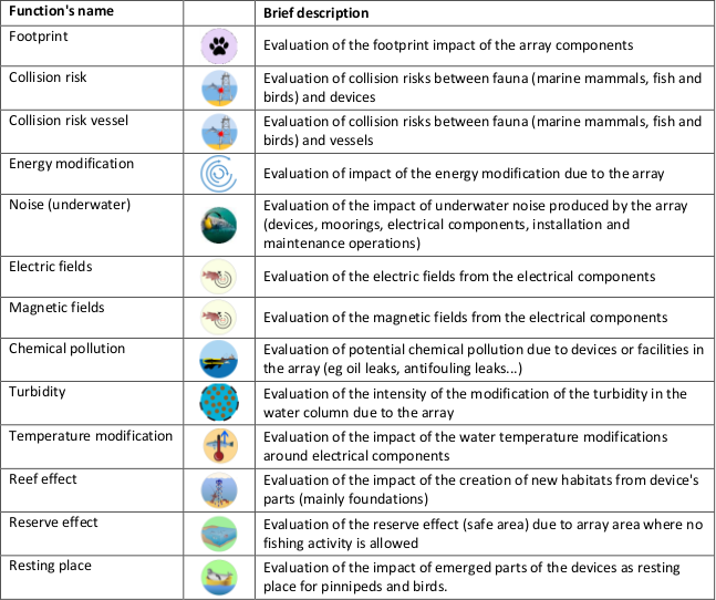
Fig. 8.25 List of environmental impacts assessed by DTOcean
Each issue is specifically allocated to the different DTOcean modules (Hydrodynamics, Electrical Sub- Systems, Mooring and Foundations…), as each module generates different stressors depending on its purpose. Fig. 8.26 shows which issues are assessed for each of the DTOcean modules. As can be seen, the computational modules with the highest number of issues are the Hydrodynamics and the Electrical Sub-Systems modules.
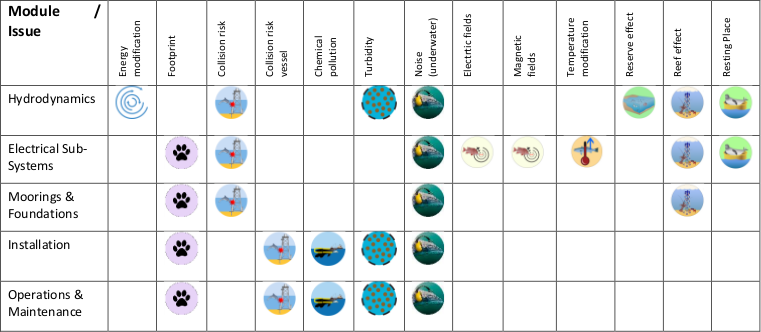
Fig. 8.26 Environmental issues associated with each DTOcean modules
Considering these issues for all the modules results in 13 specific environmental functions, with specific input values depending on the module. These functions quantify the pressure generated by the devices and their components.
8.3.4. Scoring System Principles
The use of environmental functions allows the EIA to generate numerical values (function’s scores) that will be converted to an EIS ranging from +50 to -100 (scale shown in Fig. 8.27).

Fig. 8.27 Example EIS scale
8.3.5. Environmental Functions Overview
In order for the user to have both a global environmental assessment and detailed information when using the DTOcean software, two levels (L1 and L2) of results will be available within the software. The relationships between the levels will also be made available. At each level, adverse and positive impacts are always given separately. The different display levels are defined as follow:
- Level 1: The first level of assessment provides a global (agglomerated) EIS given for each module. The result for each module is generated by the summation of EIS obtained by each function selected for that specific module and normalised on the scal e ranging from +50 to -100. This level also contains the range of impacts associated with the EIS for each module. A graphical example of the level 1 results is given in Fig. 8.28.
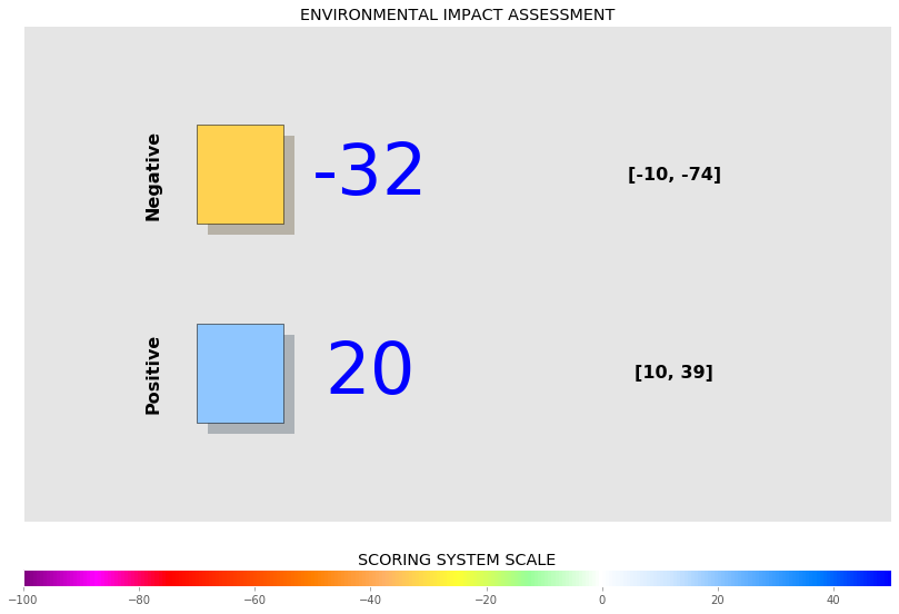
Fig. 8.28 Illustration of the module environmental impact score display
- Level 2: The second level provides full details at the function level. This level also contains the level of confidence associated to the EIS for each function. A graphical illustration of this level is shown in Fig. 8.29.
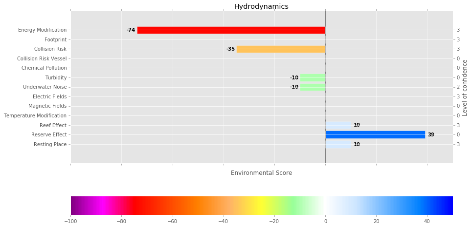
Fig. 8.29 Illustration of the function environmental impact score display
By default for the summation purpose (going from L2 to L1), all functions and modules have the same weight. However, the user will have the possibility to weight the function differently if needed.
8.3.6. Software requirements
The scoring allocation system developed within the EIA is generic for each environmental function and is shown in Fig. 8.30. The main principle for the different steps is summarised below and is based on three main steps:
STEP 1: quantification of the ‘pressure’ generated by the stressors
The quantification of the pressure is obtained from the environmental functions selected and the produced Pressure Score (PS). The PS is then adjusted to a new numerical value called the Pressure Score adjusted (PSa) through a ‘weighting protocol’ by multiplying the PS with a coefficient ranging from 0 and 1. This happens if local environmental factors exist, which are independent from the receptors, and are not included in the function’s formula. If no weighting is selected, a default value of 1 used.
At this stage the level of confidence is at its lowest value of 1.
STEP 2: basic qualification of the occurrence (or absence) of receptors
The second step is triggered if the user is able to indicate the existence of receptors onsite. Step 2 uses the score initially generated in step 1 and then adjusts it depending on the receptor’s sensitivity by multiplying the PSa with the Receptor Sensitivity coefficient (RS), which ranges from 0 to 5, unless the user has no receptor data, in which case the RS is assumed to be at its maximum value 5. This process leads to the Receptor Sensitivity Score (RSS). The different receptors are gathered within main classes reflecting their sensitivity to pressure. The user will have to choose between these different main classes of receptors that will be characterised by having RS values ranging from 0 to 5 for low to high sensitivity, respectively. When several receptors are identified onsite, the most sensitive receptors will be considered for the EIS calculations. To ultimately obtain the EIS a linear mapping is applied and specific calibration tables are used to convert RSS to EIS. In the case where the user declares a receptor that is regulatory protected (list provided by the database), by default this will automatically lead to an EIS of -100.
If the user is able to provide details about the existence of receptors, the level of confidence increases to medium, corresponding to the value 2.
STEP 3: qualification of the seasonal distribution of receptors
The last step is triggered if the user has monthly data for the existence of receptors onsite. The step then modulates the final EIS to take into account less sensitive receptors when the highest sensitive receptors are declared absent. Step 3 is similar to step 2 for each specific receptor declared onsite and the EIS is equal to 0 for any receptors absent in a particular month. For each month, the EIS is given by the most sensitive species present.
If the user has such monthly data, the level of confidence is at its highest value of 3.
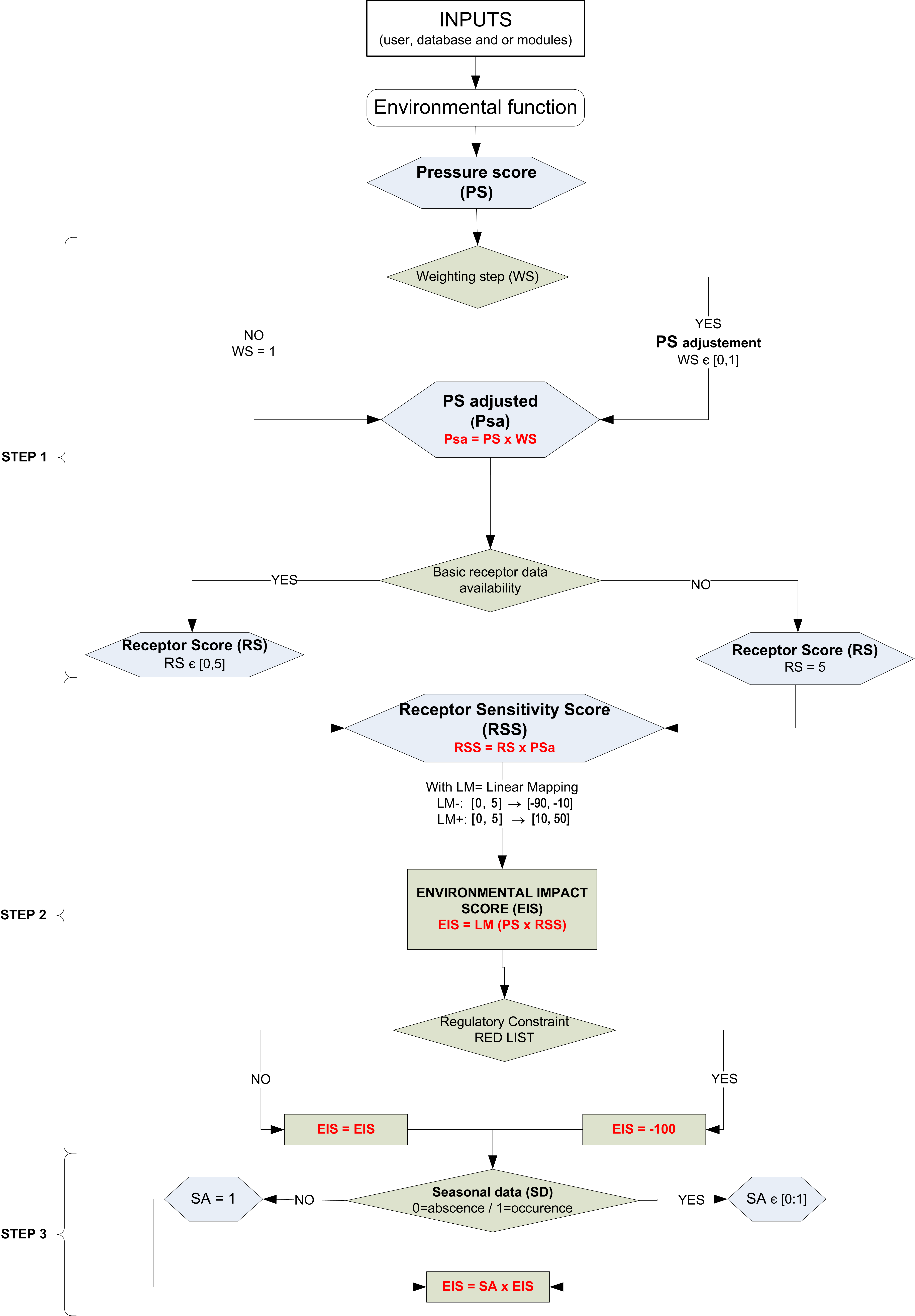
Fig. 8.30 Scoring algorithm for the Environmental Impact Assessment (EIA)
8.3.6.1. Lists used for Calibrations
Environmental scores (receptors, weighting, seasonal) have been defined using different lists of parameters according to the list presented in Fig. 8.31.

Fig. 8.31 List of scoring parameters used in the environmental assessment
8.3.6.2. Description of Environmental Functions
All of the functions are described in this section. The description is based on a generic template that includes all of the different items associated to the function. Fig. 8.32 presents the generic items described for each function.

Fig. 8.32 Details on function explanation

Fig. 8.33 Environmental parameters of the array layout module
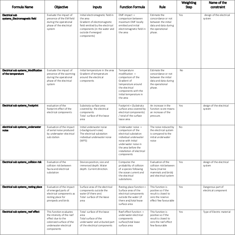
Fig. 8.34 Environmental parameters of the electrical sub-system module

Fig. 8.35 Environmental parameters of the Moorings and Foundations module

Fig. 8.36 Environmental parameters of the Installation module

Fig. 8.37 Environmental parameters of the O&M module
8.3.7. Architecture
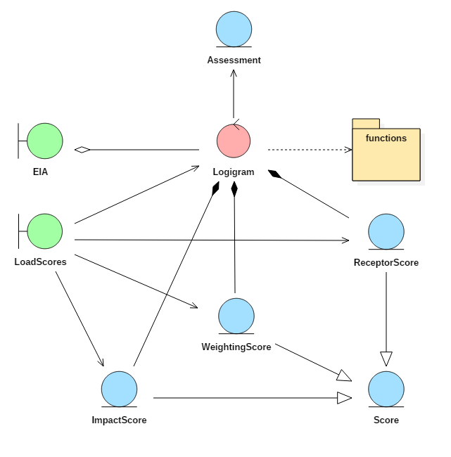
Fig. 8.38 Robustness diagram for the environmental assessment module
The implementation of the requirements detailed in this section is shown in Fig. 8.38. The main component of this system is the Logigram class that creates a programmatic representation of the flow chart shown in Fig. 8.30. A single subclass of the Logigram class exists for each environmental function detailed in the previous section. These are loaded from a module containing all the programmatic definitions of the function, the module being called the same.
Each Logigram contains three subclasses of the class Score. A score class contains a Python pandas table that carries all the scores which are used to amalgamate the result of the environmental function result and the observations of receptors or other sensitive items that weight of the function output. The column names of the tables in each Score subclass can vary, so it is the responsibility of the subclasses to check the format of the entered data.
The values for these tables are retrieved from files which are stored alongside the source code for the module (in JSON format, for instance). It was chosen to store these values locally, rather than in the global database as the values are extremely sensitively balanced and modification by an unexperienced user would be undesirable. A special boundary class called LoadScores is available to help collect the scores from the files and load them into Logigram classes.
The EIA boundary class is used to trigger each Logigram subclass as required. As the volume of input data can vary depending on which modules are run, the Logigram classes contain an abstract property called “trigger_identifiers” which returns a list of identifiers (related to the definitions of the functions, not the DDS) that can be accessed by the EIA class. As the input data to the EIA is given in the form of a dictionary, it can check the identifiers against each of the Logigram subclasses it contains and activate them as appropriate.
Each Logigram produces an Assessment class to store its results and these are returned to the EIA class following execution. The EIA class then has methods to amalgamate the results related to the type of impact (see Table 7.6) and create an overall global assessment. The user of the software can then access each of these various levels of information.
8.3.8. Functional Specification
The following section considers setting up Logigram classes, executing them independently and then executing them together through an EIA class.
8.3.8.1. Creating a Logigram subclass
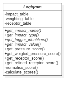
Fig. 8.39 UML class diagram for the Logigram class
A single Logigram class can be prepared for completing an isolated assessment for one function as defined in Appendix L. A UML class diagram of the abstract Logigram class is given in Figure 7.15. To create a concrete class for a specific function, four methods must be overloaded. An example of supplying these methods for the energy modification function is shown in Figure 7.16. Although this process has already been completed for all the functions required for the DTOcean software, it is useful to see that extending these functions is a straightforward process.
from .functions import energy_mod

...

def get_impact_name(self):
   return “Energy Modification”

def get_impact_type(self):
   return “Energy Modification”

def get_trigger_identifiers(self):
   indentifiers = ["input_energy",
                   "output_energy",
                   "seabed_observations"]
   return identifiers

def get_impact_value(self, inputs_dict):
   result = energy_mod(inputs_dict["input_energy"], inputs_dict["output_energy"])
   return result
8.3.8.2. Initialising a Logigram subclass
Once a concrete subclass of the Logigram class is created it must be initialised with data representing the scoring of each component of the flow chart shown in figure 7.4.5. These scores are collected in subclasses of the Score class, in order to ensure the format of the given data is correct. For example, building an ImpactScore class is undertaken as follows:
impact_score_dict = {"impact": [ 0., 0.1, 0.2, 0.3, 1.],
                     "score": [ 0., -1, -3, -5, -5], }

impact_score = ImpactScore(impact_score_dict)
The process is similar for creating the WeightingScore and ReceptorScore objects, ensuring that the correct columns are given. Once these three objects are created, it is straightforward to initialise the Logigram class, as so:
energy_modification = EnergyModification(impact_score,
                                         weighting_score,
                                         receptor_score)
As with the definitions of the Logigram subclasses, it is not anticipated that a standard user would wish to modify the scores provided alongside the code. Should they wish to load a Logigram subclass with the stored values, a helper class is provided called LoadScores. The LoadScores class uses a path to the location of the stored files. The resulting objects takes an uninitialised Logigram subclass and return an initialised object containing the stored score values. A default path for the score file will also be stored within the LoadScores class, making it very easy to use. For example, to initialise an EnergyModification object requires just the following code:
loader = LoadScores()
energy_modication = loader(EnergyModification)
8.3.8.3. Executing a Single Logigram
Executing a Logigram object is simply a matter of supplying the necessary inputs. The input relating to the specific impact is unique to the Logigram subclass being used; however the inputs are always entered in a similar manner, using a Python dictionary. Additionally, a list of observed protected species and a dictionary containing observations for species subclasses can be given. The keys of this dictionary relate to the subclass itself, and the values allow per month observations. If these monthly observations are not known then the value “None” indicates they are known to be present, but it is not known when they are present. Using the EnergyModification Logigram subclass as an example once again, the process for executing it, using the energy_assessment object that was made earlier, would be as follows:
impacts = {"input_energy": 100,
           "output_energy": 90,
           "seabed_observation": "Loose sand"}

protected_observations = ["clown fish"]

subclass_observations = {"soft substrate ecosystem": None,
                         "particular habitats": ["Jan", "Feb", "Mar", "Apr"],
                         "benthos": ["Jan", "Feb", "Mar", "Apr"] }

energy_assessment = energy_modification(impacts, protected_observations, subclass_observations)
The output of the call to the energy_modication object is an object of the Assessment class. This class standardises the outputs of the assessments so they can be combined easily. In general, they contain the following attributes:
- impact_type: the class of impact which contains this function
- score: the combined score for the function (+ve or –ve depending on the type)
- confidence_level: the level of confidence depending on the known data
- impact_scores: a dictionary detailing the impact score calculation
- protected_scores: a dictionary detailing the scores for protected species
- basic_receptor_scores: a table detailing the scores relating to non-temporal subspecies observations
- temporal_receptor_scores: a table detailing the scores relating to temporal subspecies observations
8.3.8.4. Using the EIA Class to Combine Impacts
The EIA class allows many Logigram subclasses to be executed at once, in response to the data available. It can also combine those assessments to produce aggregated scores for impact types and an overall score for all of the impacts.
An EIA class can be initialised with a list of Logigram subclass objects which have been initialised as described above. This EIA class is then ready to use in a very similar manner to the individual Logigram subclasses, except that the impacts dictionary is expanded to include all of the variables that relate to impact scores. An example of creating and executing an EIA class object is as follows:
environmental_assessment = EIA([energy_assessment,
                                seaborn_impact_risk, ... ])

all_assessments = environmental_assessment(impacts,
                                           protected_observations,
                                           subclass_observations)
The output “all_assessments” is a dictionary where the keys are the name of the impact (retrieved with the “get_impact_name” method) and the values are the Assessment objects related to that particular impact. The EIA class has three further functions for amalgamating the assessment scores. These are:
- type_scores: generates scores and confidence levels per impact type
- local_score: generates a total score and confidence level for a single module
- global_score: generates a global total score for all the modules
The first two functions take the dictionary output of the EIA call (all_assessments), but the last function takes a list of all the local scores which are required to be combined into the overall global assessment.