7. DTOcean Modules¶

7.1. Hydrodynamics Module¶

7.1.1. Requirements¶

7.1.1.1. User Requirements¶

The scope of the Hydrodynamics module is the identification of an array configuration that maximizes the AEP of the array, while holding the average q-factor of the array above a user specified threshold. The q-factor is an energy losses index, definable as the modification of the absorbed energy due to the hydrodynamic interaction between bodies. It is calculated as the AEP of the array over the AEP of the same array without considering the interaction.

The package solves the hydrodynamic interaction between OEC devices in the array and, based on the solution of the hydrodynamic problem, the energy extracted by each device. The latter is in turn used to estimate the q-factor for the array.

The AEP is used as the convergence criterion within the optimization loop. The optimization parameter space is defined by the array parameters, such as device inter-distance, rows and columns angles, etc. The parameter space is continuous and real-valued.

The optimum search is constrained by the following variables: the no-go areas, the minimum distance between devices, the maximum number of devices and the q-factor.

7.1.1.2. Software Design Requirements¶

The core of the package is divided into two sub-packages, namely tidal and wave. This subdivision is driven by the different way of solving the hydrodynamic interaction.

The tidal sub-package solves the hydrodynamic interaction between turbines using a parametrized look-up table to describe the wake shape and solving the wake interaction based on the semi-empirical models inherited from the wind sector. The wakes are placed in the array area based on the estimation of the streamlines evaluated using Lagrangian drifters at the turbines locations. The wake shape look-up table is populated from CFD runs.

The wav esub-package solves the hydrodynamic interaction within the array using the so-called direct matrix method. The method uses the cylindrical coordinate description of the wave field generated by the presence of the moving device, and maps it to the global array coordinate system. The solution of the hydrodynamic problem in the cylindrical coordinate system is obtained by solving the Laplace equation in the fluid domain, using a boundary element method solvers.

For a detailed description of the mathematical formulation of the hydrodynamics algorithms see (Silva, et al., 2015).

7.1.2. Architecture¶

At a high level the Hydrodynamics module is divided into two blocks: the main routine where the pre-processing is carried out and an optimization routine where the actual array optimization is performed. The top level view of the code is simplified in Fig. 7.38.

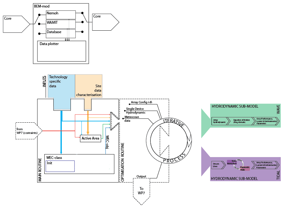
Fig. 7.38 Hydrodynamic model top level view.

The main routine collects the inputs and evaluates the following quantities:

The Active Area is defined as the no-go areas subtracted from the lease area

WEC hydrodynamic (only for wave energy converters) evaluates the hydrodynamic properties of the device in the local cylindrical coordinate system

WEC fitting (only for wave energy converters) tunes the numerical model to the user provided power performance of the device. It corresponds to the green box “single body performance fit” in Fig. 7.38

Additionally, the routine requires two objects; a Hydro and an Array class object:

The Hydro class object collects the metocean conditions that describe the features of the site, i.e. bathymetry, sea state description, etc.

The Array class object is used to generate the grid layout given the array type and the parameters value, and to identify which devices are inside the active area. A check on the minimum distance constraint is performed too

The optimization routine calls either the tidal or wave submodule, for the resolution of the array interaction problem, given the required inputs.

7.1.2.1. Modules and functions description¶

The detailed description of the programmatic structure of the Hydrodynamic module is given hereafter; a graphical representation is given in the Unified Modelling Language (UML) diagram presented in Fig. 7.39.

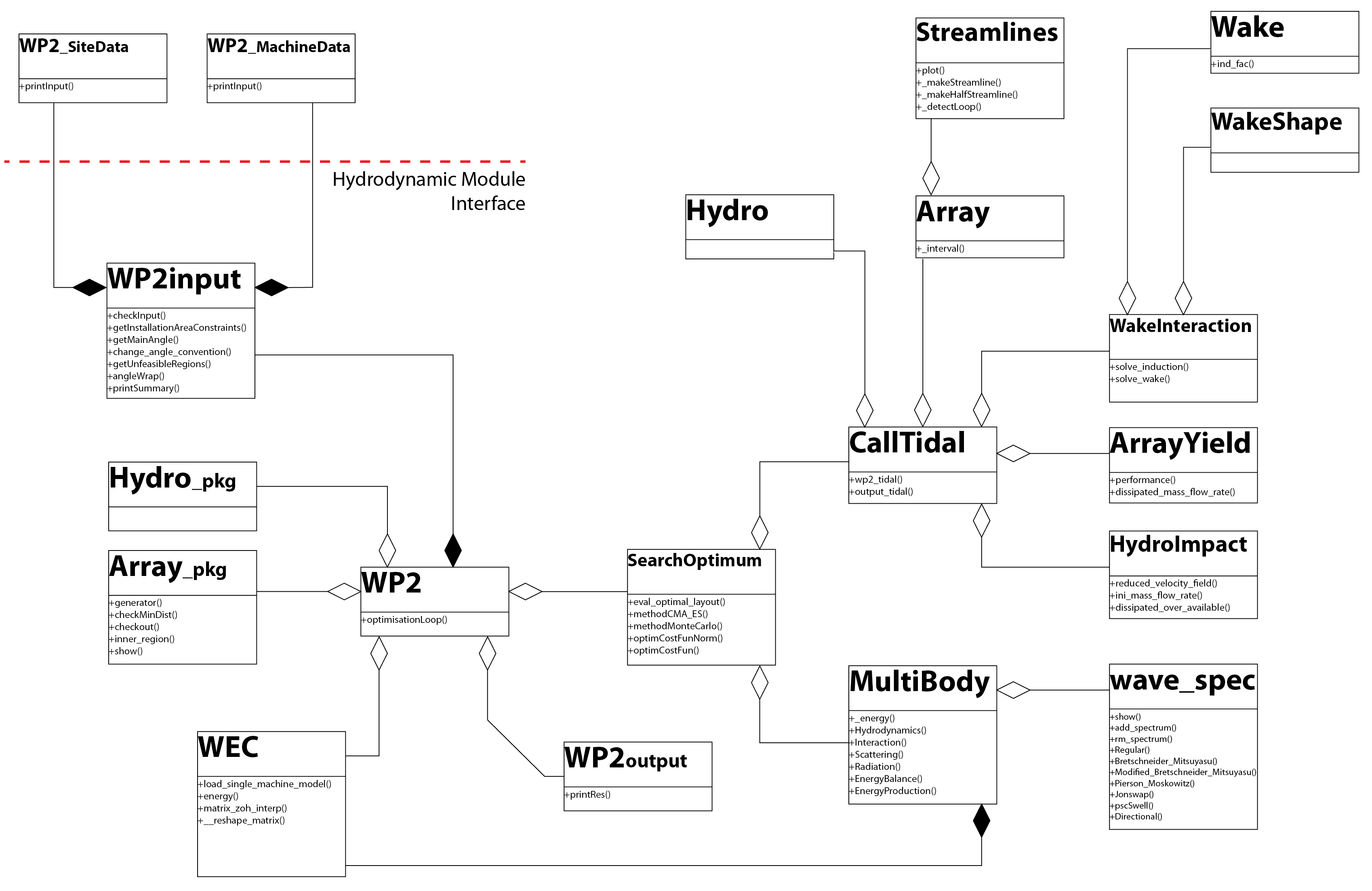
Fig. 7.39 UML diagram of the Hydrodynamic model.

WP2input:

The WP2input class is composed of two further classes, WP2_SiteData and WP2_MachineData.

These classes contain the features of the development site and the actual machine, respectively. Their role is passive since they are used as structured data containers. The WP2_SiteData and the WP2_MachineData objects will be initialised independently and so a line could be drawn between those objects and WP2input (see Fig. 7.39) illustrating the starting point for the WP2.

On the contrary, a WP2input object will perform a series of tasks at the initialisation.

Check if the inputs conformed to the input requirements. If step (a) returns 0, i.e. inputs are correct, then:

Map the angles into the hydrodynamic model format. The wave metocean conditions are given with angles defined in the reference system: South – West, while for the sake of simplicity the

Hydrodynamics module uses the convention East – North. The conversion is made at the input level in order to avoid any confusion later in the process

Identify the main angle, which is used for the array orientation. This will define the rotation matrix around the vertical axis. The main angle is extracted from the MainDirection, which is in turn given by the user in form of Easting-Northing components, or calculated from the sea state with the highest probability of occurrence. For the wave case the probability of occurrence is ranked applying the summation over the wave height and wave period axis

Identify the polygons where the devices cannot be installed due to installation constraints dictated by the water depth. The method first checks for two trivial solutions, such as no feasible installation points and all feasible installation points. If none of the trivial solutions are present, the algorithm will:

Identify the feasible and unfeasible installation points in the given bathymetry

Cluster the unfeasible installation points using a density based method

Identify the bounding polygons for each cluster (no-go area)

Test if the polygon has some feasible point inside, and if that is the case identify the bounding polygon of the feasible area inside the unfeasible area

The generated WP2input object is then using to create a WP2 object at the instantiation using a composition scheme.

WP2:

The WP2 class is the main controller class of the hydrodynamic model. It initializes the Hydro class as well as the Array class (aggregation), which are used all the way through the output generation. For the case of an array of WECs, the WEC class is also instantiated. The WEC class is used to assess the hydrodynamic features of a single WEC, which define the base for the solution of the array interaction problem. Within the optimisationLoop method, the WP2 class conditionally instantiates a search optimum object that encapsulates the optimization algorithm or generates a solution for the given array layout. The type of array grid specified by the user leads the decision. This option gives the user the freedom to specify an array layout or let the software decides the best one.

At the completion of the work the WP2 class returns a WP2output object.

Hydro_pkg:

The Hydro_pkg class collects the information about the sea states of the site, their probability of occurrence as well as the bathymetry and the sea surface height at the given grid points.

The class can be considered to have an entity stereotype since it is used as a structured data container.

Array_pkg:

The Array_pkg class collects the information of the active area, the main orientation angle, and the minimum allowable distance between devices. The active area is built from a Boolean intersection between the Lease Area and the no-go areas.

An object is used in the optimization call, to generate an array layout, to check on the feasibility of the given layout and to mute all devices that do not belong to the Active Area.

The generation of the array layouts is based on the input grid structure type; possible alternatives are:

Rectangular grid: perpendicular angle between rows and columns, and variable rows and columns distances

Staggered grid: equal distance and angle between rows and columns; the angle can vary in the range 0-90 degrees

Full grid: variable rows and columns distance and variable rows and column angles

Prior to the evaluation of the array interaction the array layout is verified against the minimum distance parameter, in order to avoid violation of that constraint. For the above-mentioned grids the check is performed on a single cell of the grid, while for a user given array layout, the check is performed sequentially for every point.

Lastly, each grid vertex is tagged with a Boolean value based on its position with respect to the Active Area. Due to the irregularity of the Active Area, the process is performed sequentially for each grid vertex.

WEC:

The WEC class is only instantiated for the case of an array of WECs and is used to load and manage the numerical model of the isolated Wave Energy.

search_optimum:

The main objective of the search_optimum class is to generate the “best” array layout given the specification of the deployment site and the single machine properties.

“Best” is defined in agreement with the cost function built into the class, which is targeted to maximize the AEP of the array, given some constraints of the feasible solutions, such as the q-factor, the minimum distance between devices or the maximum number of devices.

The search_optimum class uses (as a default option) a heuristic optimization approach, of the Evolutionary Strat- egy type, to identify the array layout that maximises the given cost function.

The parameter space order depends on the type of grid layout specified; therefore a mapping rule between full and reduced order spaces is generated. Then, the reduced parameter space is scaled so that the range of values is the same regardless of the parameter.

The search algorithm is based on the concept of natural genetic evolution, where the actual population holds the genes of the previous winner elements, and additional randomness is brought by introducing random seeds in the generation process. This is achieved by searching the optimum in the region defined by the mean value plus and minus three standard deviations of the current population. The mean and the standard deviation are weighted so that the best specimens have more weight than the rest.

Each element of the population represents a different array layout, which hydrodynamic interaction needs to be solved. The search_optimum class instantiates either a CallTidal (in the tidal case) or a MultiBody (in the wave case) object. The objects use the information of the array layout stored in the Array object and the features of the single device to generate an array of devices and solve their interaction.

For a more detailed description of the optimization algorithm the reader is referred to (Silva, et al., 2015).

CallTidal:

The CallTidal class is an interface class used to query the wp2_tidal function, given the device position, the machine specification and the site specification. Superimposing the site velocity field with the single machine one solves the hydrodynamic interaction. The single machine velocity field is based on a parameterized wake database (distributed along with the Hydrodynamic module), and the wake is located in the global coordinate system based on the device position and the calculated streamline. The wp2_tidal method instantiates an Array, a Hydro, a WakeInteraction, an ArrayYeld and a HydroImpact object, which solve the interaction problem.

Array:

The Array class contains the information about the spatial distribution and the hub velocity of the devices in the array and calculates the shape of the streamlines for each device based on the velocity field of the area. The class aggregates a number of streamline objects, one for each device, used to calculate the streamline shape from the device position.

Stramlines:

The Streamlines class is used to calculate the streamline shape, giving the velocity field of the area and the initial position. The algorithm uses a Lagrangian drifter approach to evaluate the streamline shape.

Hydro:

The Hydro class contains the features of the site, such as velocity field, bathymetry and geophysical information of the seabed.

The Hydro class has an entity stereotype since it is used primarily as a structured container for the site data. WAKEINTERACTION:

The WakeInteraction class encapsulates the main algorithm to assess the hydrodynamic interaction in the array. It uses the Wake and the WakeShape classes to store and to map the single machine shape into the global ve- locity field of the area. The resultant velocity field is obtained through an iterative process, which involves the superimposition of the wakes and the recalculation of the wake shapes for the new velocity field.

Wake:

The Wake class stores the 2D map of the velocity field around the machine, for the given input conditions. The Wake queries a precompiled database with the following entry points: thrust coefficients, turbulence intensity, yaw angle and blockage ratio. The query is handled by FORTRAN code which is precompiled as a Python extension module.

WakeShape:

The WakeShape class calculates the wake shape in the global coordinate system, given a Wake object, the machine features and the streamlines previously calculated.

ArrayYeld:

The ArrayYeld class is instantiated after the solution of the array interaction and is used to calculate the power performance of each machine, given the machine features and the hub velocity. It also assesses the dissipated mass flow rate through the machine.

HydroImpact:

The HydroImpact class is instantiated after the solution of the array interaction and the calculation of the array yield. It uses the dissipated mass flow rate through the machine to assess the modification of the velocity field induced by the array. This parameter is used to assess the environmental impact of the array.

Multibody:

The Multibody class is the wave counterpart of the CallTidal object. It is used to build an array of WECs and to solve the hydrodynamic interaction within the array.

The generation of the array of WECs is based on the array layout coordinates and on the single machine features, which are stored in the WEC object. The WEC object is a prerequisite of the Multibody and is generated by the WP2 object in the pre-processing phase. The Multibody class generates a numerical model of the array using the direct matrix method, and evaluates the energy production of the array based on the site features; in particular the definition of the sea states and their probability of occurrence are used in this step.

During the energy assessment the Multibody class generates an instance of the Wave_spec class.

Wave_spec:

The Wave_spec class is used to generate a parameterised wave energy distribution over the spectrum of frequency and directions. It supports all the commonly used types of frequency spectral models, such as the JONSWAP and Pierson-Moskowitz (PM) spectra.

WP2output:

The WP2 class issues the WP2output object after the search of the “best” array configuration is completed. The class has an entity stereotype.

7.1.3. Functional Specification¶

7.1.3.1. Inputs¶

In order to use the Hydrodynamics module the first step is the generation of WP2_SiteData and WP2_MachineData objects, which contains all the information needed by the module to run.

The WP2_SiteData object has a series of ten inputs listed hereafter:

LeaseArea (numpy.ndarray) [m]: the area where the machines can be installed

NogoAreas (list) [m]: the area where the machines can NOT be installed within the “LeaseArea”

MetoceanConditions (dict): sea state definitions: the format is strictly related to the machine type (wave or tidal)

VelocityShear (numpy.ndarray) [-]: the power law exponent to be used in the definition of the vertical velocity profile

Main_Direction (numpy.ndarray, optional) [m]: the main direction of the array. The array will be aligned with this direction and the optimization parameter space will be defined around it. If a None value is passed, the model evaluates the main direction from the probability of occurrence of the different sea states

Bathymetry (numpy.ndarray) [m]: the seabed profile of the lease area, the datum is not important but it needs to be in agreement with the SSH parameter specified in the MetoceanConditions parameter

Geophysics (numpy.ndarray): the Manning number of the area, specified at each grid point. The value is used along with the VelocityShear to assess the vertical velocity profile.

BR (float) [-]: the horizontal blockage ratio, the ratio between the lease area and the channel area. A BR of 1 identifies a closed boundary lease area, while a BR of 0 identifies an open water scenario

electrical_connection_point (numpy.ndarray) [m]: UTM coordinates of the electrical connection point at the shore line, expressed as [X(Northing),Y(Easting)].

boundary_padding (float, optional) [m]: Padding added to inside of the lease area in which devices may not be placed

Similarly the WP2_MachineData object contains a list of nineteen inputs, of which eight are optional, listed hereafter:

Type (str) [-]: either “wave” or “tidal”. The variable will trigger the different routines in the model

lCS (numpy.ndarray) [m]: position of the local representative point of the machine in the 3D space. For a wave case it is the position of the device centre of gravity seen from the mesh coordinate system. For a tidal case only the third (vertictal) coordinate is used to identify the position of the hub from the reference point. For a floating machine the reference point is the sea surface elevation, while for a bottom fixed machine it is the seabed

Clen (numpy.ndarray) [m]: (used only for a tidal case) the rotor diameter and the distance from the centre line. If the distance from the centre line is bigger than zero, a double rotor machine will be considered

YawAngle (float) [rad]: the yawing angle span of the machine, which describes the self-orienting capability of the device

Float_flag (bool): whether the machine is bottom fixed or floating

InstallDepth (list) [m]: the water depth range where the machine can be installed. All the points in the lease area which are not contained within the given range are grouped into nogo areas

MinDist (tuple) [m]: the minimum distance between devices in the array. For the wave case, the minimum distance is given by the circle that inscribed the machine, and this condition is enforced if the user specifies a smaller distance

OpThreshold (float) [-]: is the minimum q-factor allowable. The input is used during the optimum search to identify the maximum accepted value of the hydrodynamic losses. Any array layout that generates a q-factor smaller than the OpThreshold will be disregarded

UserArray (dict): identify the type of array layout to be evaluated, based on the Option parameter. If option 1 is chosen, one of the specified array layouts will be optimised. Possible choices are ‘Rectangular’, ‘Staggered’ and ‘Full’. If option 2 is selected, the given array layout, specified in the value variable, is solved without optimisation. If option 3 is selected then the given array layout is optimised based on a simple homogeneous compression/expansion

RatedPowerArray (float) [W]: the target rated power of the array. This is used to bound the optimisation search

RatedPowerDevice (float) [W]: the rated power of the machine

wave_data_folder (string, optional): path name of the hydrodynamic results generate by the wave external module

tidal_power_curve (numpy.ndarray, optional)[W]: Power curve function of the stream velocity

tidal_trust_curve (numpy.ndarray, optional)[Nm]: Trust curve function of the stream velocity

tidal_velocity_curve (numpy.ndarray, optional)[m/s]: Vector containing the stream velocity

tidal_cutinout (numpy.ndarray, optional): contain the cut_in and cut_out velocity of the turbine. Outside the cut IN/OUT velocity range the machine will not produce. The generator is shut down, but the machine will still interact with the others.

tidal_bidirectional (bool, optional): bidirectional working principle of the turbine

tidal_data_folder (string, optional): Path to tidal device CFD data files

UserOutputTable (dict, optional): dictionary of dictionaries where all the array layouts inputed and analysed by the user are collected. Using this option the internal WP2 calculation is skipped, and the optimisaton is performed in the given data. The dictionaies keys are the arguments of the WP2 Output class.

7.1.3.2. Execution¶

In the following, the sequence of commands to run the WP2 is given:

>>> i = WP2input(Machine, Site)
>>> WPobj = WP2(i)
>>> Out = WPobj.optimisationLoop()

Machine is an instance of WP2_MachineData and Site is an instance of WP2_SiteData, both must be initialized before WP2 can take place.

The variable Out is an instance of the class WP2output, with attributes the ones listed in the previous section.

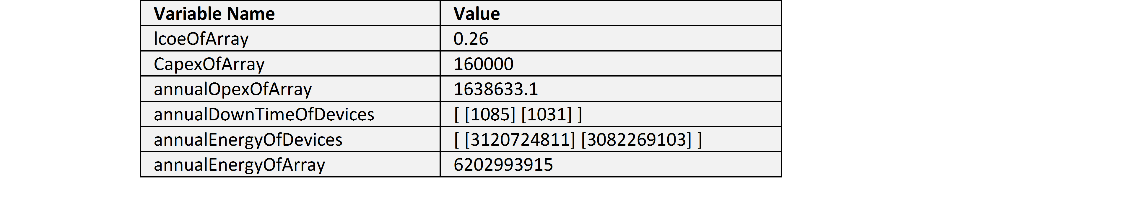
7.1.3.3. Outputs¶

As introduced previously the Hydrodynamic module will return an output object at the end of the run with the following attributes:

AEP_array (float)[Wh]: annual energy production of the whole array

power_prod_perD_perS (numpy.ndarray)[W]: average power production of each device within the array for each sea state

AEP_perD (numpy.ndarray)[Wh]: annual energy production of each device within the array

power_prod_perD (numpy.ndarray)[W]: average power production of each device within the array

Device_Positon (numpy.ndarray)[m]: UTM coordinates of each device in the array. NOTE: the UTM coordinates do not consider different UTM zones. The maping in the real UTM coordinates is done at a higher level.

Nbodies (float)[]: number of devices in the array

Resource_reduction (float)[]: ratio between absorbed and incoming energy.

Device_Model (dictionary)[WAVE ONLY]: Simplified model of the wave energy converter. The dictionary keys are:

wave_fr (numpy.ndarray)[Hz]: wave frequencies used to discretise the frequency space

wave_dir (numpy.ndarray)[deg]: wave directions used to discretise the directional space

mode_def (list)[]: description of the degree of freedom of the system in agreement with the definition used in WAMIT taking in consideration only translational degrees of freedom

f_ex (numpy.ndarray)[]: excitation force as a function of frequency, direction and total degree of freedoms, normalised by the wave height. The degree of freedoms need are only the three translation defined in the mode keys.

q_perD (numpy.ndarray)[]: q-factor for each device, calculated as energy produced by the device within the array over the energy produced by the device without interaction

q_array (float)[]: q-factor for the array, calculated as energy produced by the array over the energy produced by the device without interaction times the number of devices.

TI (float)[TIDAL ONLY]: turbulence intensity within the array

power_matrix_machine (numpy.ndarray) [WAVE ONLY]: power matrix of the single WEC.

main_direction (numpy.ndarray): Easing and Northing coordinate of the main direction vector.

Independently from the type of machine or simulation selected, the results summarise the array layout and the power/energy performance of each machine. In the following figures the results of the optimisation routine are illustrated.

Fig. 7.40 shows the resultant array layout along with much other information. The results are generated for a WEC array, composed of heaving cylinders. The waves are travelling from West to East.

The red lines identify the lease area polygon, and the blue shaded areas identify the nogo areas specified by the user. As mentioned previously the active area is the Boolean difference between the two areas.

The installed machines are represented by blue dots and tagged with the corresponding ID number. The grey crosses represent grid points that are not inside the active area. The Array_pkg object generates those points, but they are not considered in the array interaction.

The arrow identifies the main direction, which corresponds to the wave direction for this case; in fact the main direction input has been set to None, in which case the software will calculate the orientation.

Fig. 7.41 represents the AEP per each device installed in the array. On the x-axis the device ID is given to define relation between the array layout and productivity in the array.

The first two rows of devices face a clean energy source, where the wave energy content has been only slightly modified. This results in a higher energy production for the first 11 devices. On the other hand, the rest of the devices receive reduced energy content and their productivity tends to be lower.

It is important to bear in mind that the WECs are not only shadowing the “down-wave” devices, therefore it can be possible to have devices in the centre of the array that benefit from the energy radiated from the circumscribing devices.

As shown in Fig. 7.42, the q-factors of the different machines are not monotonically decreasing in the Easting direction, as one could expect from a shadowing model. The figure presents the q-factor for each device as an additional vertical axis superimposed on the array layout plot presented in Fig. 7.40.

In simple words, the second rows of devices are taking advantage of a clean energy source that has been boosted by the waves radiated by the first row of devices. On the contrary, the rear rows of devices receive a scattered wave field, which reduced their hydrodynamic efficiency if compared with the isolated case.

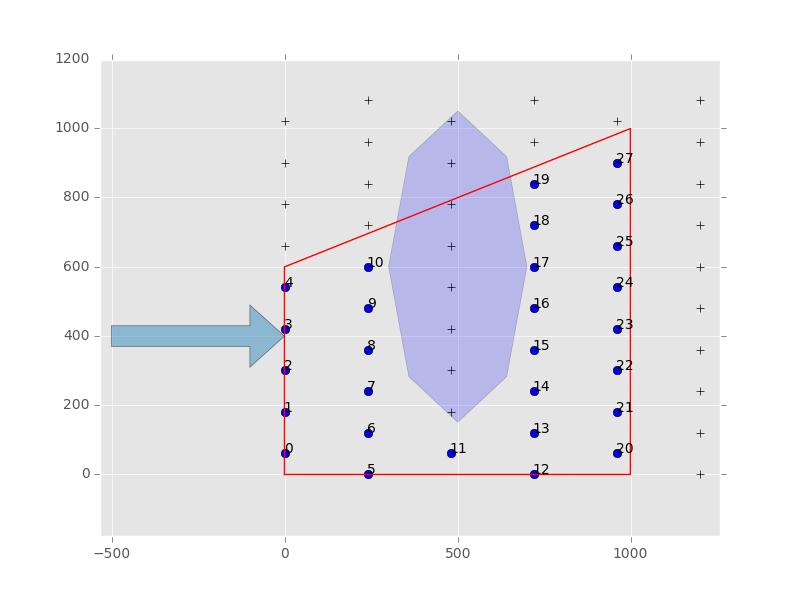
Fig. 7.40 Array layout. Installed machines (blue dots), unfeasible installation points (grey crosses), lease area (read polygon), user given nogo areas (blue area), main direction (blue arrow).

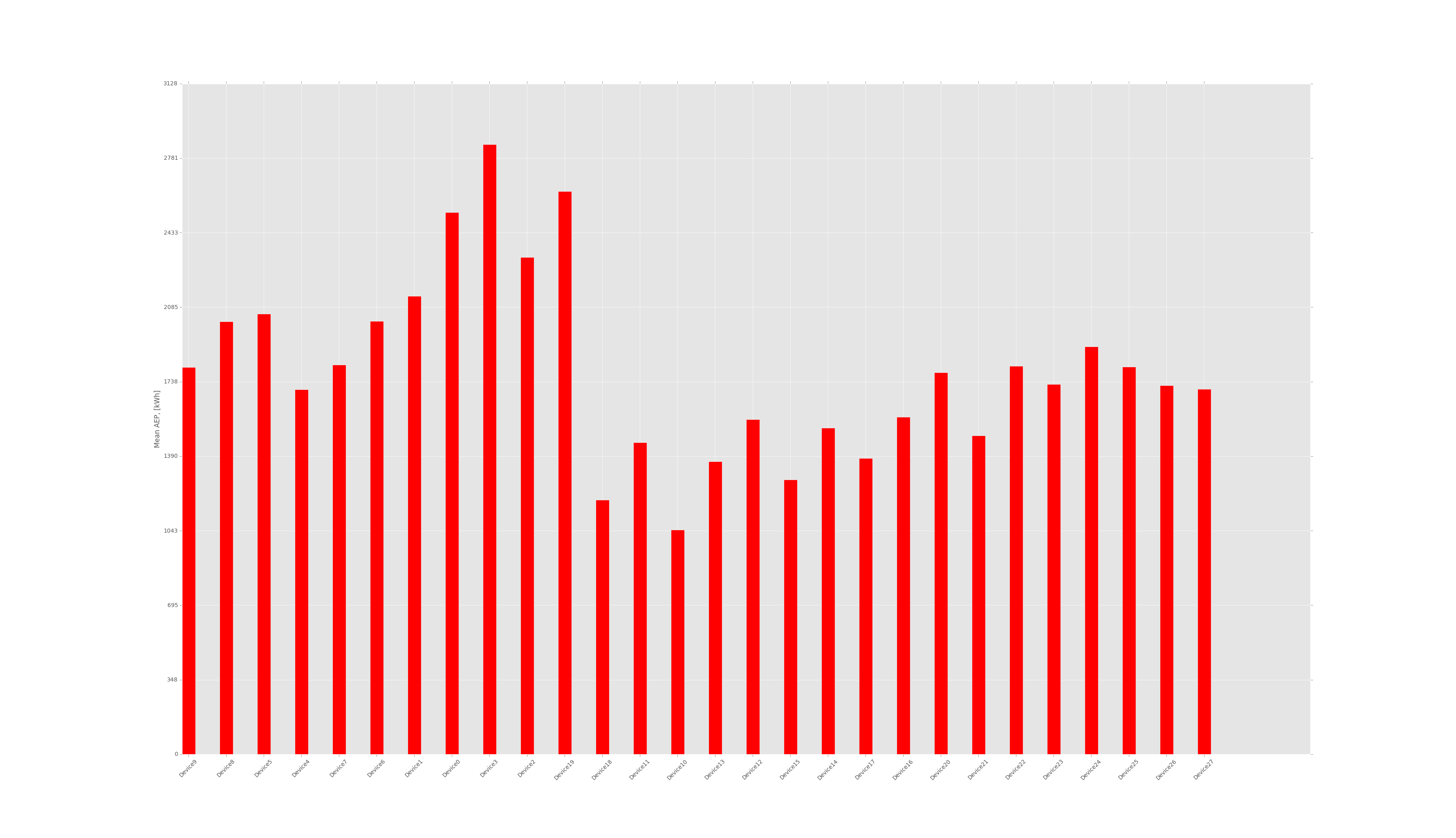
Fig. 7.41 Mean AEP for each device expressed in kWh.

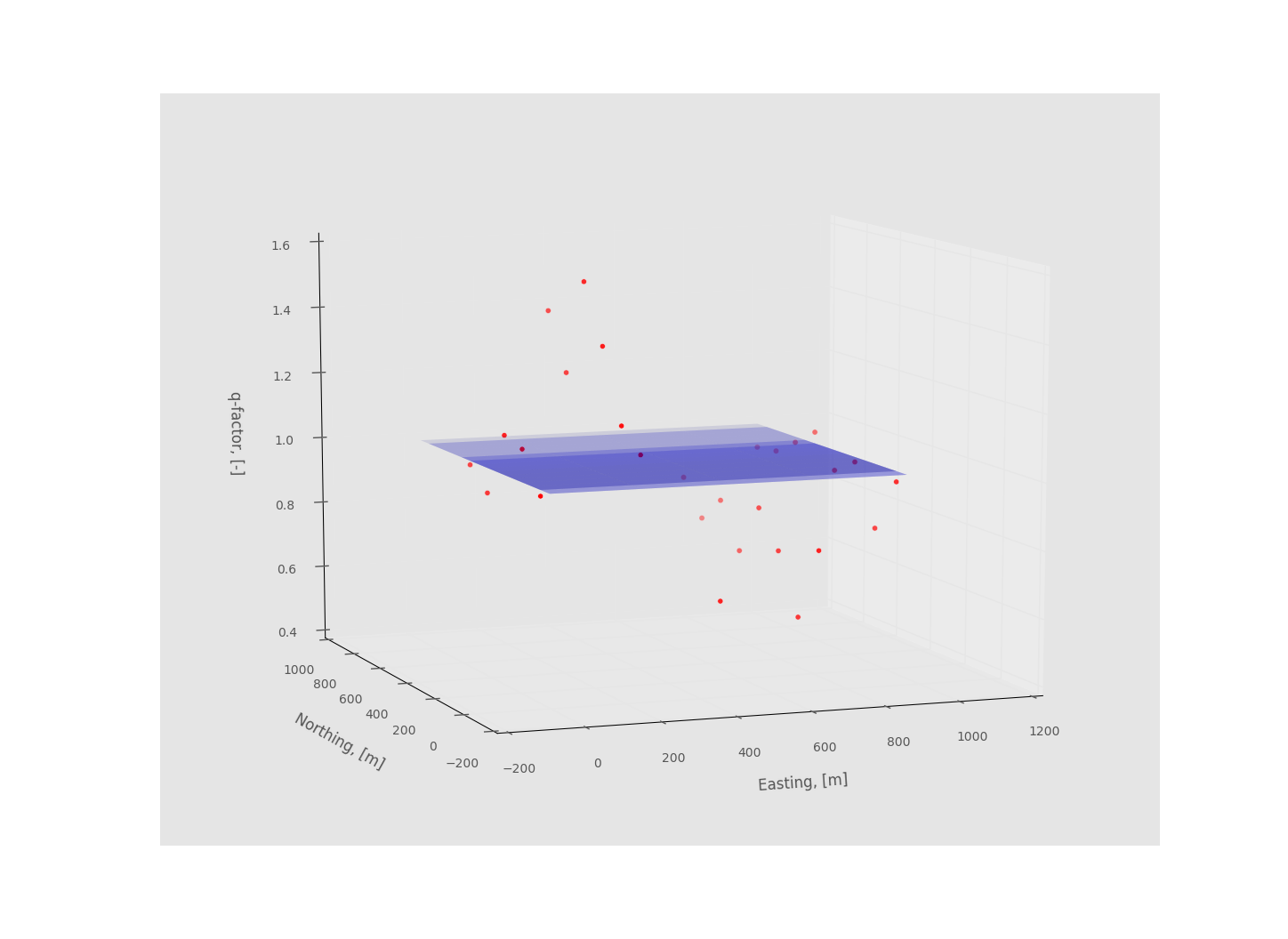
Fig. 7.42 q-factor variation in the array.

References

Silva, M., Raventos, A., Teillant, B., Ferri, F., Roc, T., Minns, N., et al. (2015). Deliverable 2.4: Algorithms providing effects of array changes on economics. WaveEC, AAU, ITP, SNL, FEM. Lisbon: EU - Commision.

7.2. Electrical Sub-Systems¶

7.2.1. Requirements¶

7.2.1.1. User Requirements¶

The purpose of the Electrical Sub-Systems module is to identify and compare technically feasible offshore electrical network configurations for a given device, site and array layout. The scope covers all electrical sub-systems from the OEC array coupling up to the onshore landing point, including: the umbilical cable, static subsea intra-array cables, electrical connectors, offshore collection points and the transmission cables to the onshore grid.

Ultimately, the network design process is defined by the following factors:

The transmission voltage, capacity and number of transmission cables;
The number, location and type of offshore collection points;
The intra-array network topology, i.e. number of OEC devices per string, number of strings, voltage level, and umbilical geometry (for floating devices);
Optimal cable routing and protection for the transmission system and intra-array cable networks.

These design criteria must be constrained by the physical environment, power flow constraints and available components. Once the solutions have been produced, a local best solution should be obtained by calculating and comparing the overall network efficiency (i.e. network losses) and component costs. The DTOcean tool remit does not consider the capital cost of onshore electrical infrastructure, but, if so desired, the user can enter a cost of these subsystems to be included when assessing the system LCOE.

7.2.1.2. Software Design Requirements¶

An offshore electrical network can be represented by a number of connected subsystems, shown in Fig. 7.43.

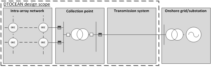
Fig. 7.43 Simplified generic offshore electrical network for OEC arrays

Network design will typically proceed from onshore to the offshore array, although some iteration between possible designs can be expected. Following this approach allows the design process to be broken down and requirements clearly defined:

Seabed processing for cable routes
Selection of suitable transmission and array voltages
Design of feasible intra-array networks
Power flow analysis of networks

The flow chart in Fig. 7.44 , based on [IET], summarises the design process.

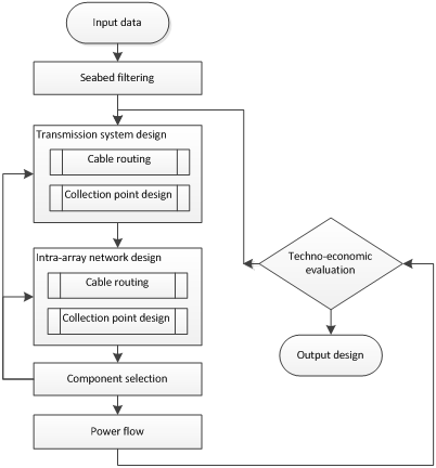
Fig. 7.44 Electrical Sub-Systems model top level view.

7.2.2. Architecture¶

The structure of the Electrical Sub-Systems module reflects the modular design approach. Seabed processing is performed prior to any electrical design in order prepare design areas. The network design stage is separated into two, with specific design processes defined for radial and star network topologies. The design work flow is unified again when preparing networks for power flow and analysis.

An overview of the structure of the Electrical Sub-Systems module is presented in Fig. 7.45.

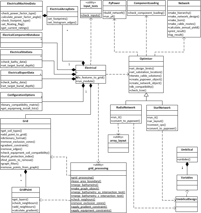
Fig. 7.45 UML diagram of the Electrical Sub-Systems model.

The python package is structured accordingly:

dtocean_electrical/
|-- dtocean_electrical/
|
|  |-- __init__.py
|  |-- main.py
|  |-- inputs.py
|  |
|  |-- grid/
|  |  |-- __init__.py
|  |  |-- grid.py
|  |  |-- grid_processing.py
|  |
|  |-- network/
|  |  |-- __init__.py
|  |  |-- cable.py
|  |  |-- collection_point.py
|  |  |-- connector.py
|  |  |-- network.py
|  |
|  |-- optim_codes/
|  |  |--_ _init__.py
|  |  |-- array_layout.py
|  |  |-- optimiser.py
|  |  |-- power_flow.py
|  |  |-- umbilical.py
|
|-- setup.py
|-- README

7.2.2.1. Overview¶

Electrical: The Electrical class is composed of six input classes: ElectricalComponentDatabase, ElectricalMachineData, ElectricalArrayData, ConfigurationOptions, ElectricalSiteData, ElectricalExportData. The input classes contain all data and data processes required to create and run an instance of the Electrical class. Upon initialisation the Electrical class will run a number of input data checks (contained in input_tests) and also align the device layout and landing point with the x-y grid.

The Electrical class also initialises the Grid class and the GridPoint class via the grid_processing utility class. Once the data has been prepared and checked, the Electrical class creates and executes an instance of the Optimiser class.

ElectricalComponentDatabase: This is a structured data container for the electrical component database. This consists of eight individual component tables for the main electrical components of an offshore network: static cables, dynamic cables, wet-mate connectors, dry-mate connectors, collection points, switchgear, transformers and power quality equipment. Each component table is stored as a pandas DataFrame object. Details of the individual fields are included in APPENDIX.

ElectricalSiteData: Define the electrical systems site data object. This includes all geotechnical and geophysical data.

ElectricalExportData: Define the electrical systems export data object. This includes all geotechnical and geophysical data.

ElectricalMachineData: Container class to carry the OEC device object.

ElectricalArrayData: Container class to carry the array object. The ElectricalMachineData object is included within this class.

ConfigurationOptions: Container class for the configuration options.

Grid: Data structure for the grid. This is composed of a number of GridPoint objects. While a GridPoint object contains only local information, a Grid object contains more useful information of the area as a complete entity. Special methods allow for creating specific design areas by removing constraints and filtering the seabed based on installation equipment functionality.

GridPoint: Data structure for grid point data. A GridPoint is created to carry the information of every x-y coordinate in the lease area and the cable corridor. For each point, neighbours are defined in either four or eight directions, with four taken by default. Spatial distances and gradients for all neighbours are calculated in order to create a series of edges and vertices for graph analysis.

grid_processing: This is utility class controls the data flow and manipulation required to convert the input geophysical and geotechnical data into the coherent dataset required by the cable routing algorithms. The processes in grid_processing are divided into three main tasks: collecting all exclusion zones, merging the lease area and cable corridor bathymetry data and creating a NetworkX graph object for cable routing analysis. The GridPoint and Grid objects are also created during this final stage, and the graph object is assigned to an attribute of the Grid class.

Optimiser: Controller class to define search space and find the network solution. This takes configuration options as constraints and searches within a predefined search space for a best solution. The search space is realised as look-up table developed with respect to the maximum power transfer of an electrical system a function of voltage and distance. These static values are compared against the spatial characteristics of the array to be designed in order to construct technically feasible voltage levels for the network. More than one voltage level is proposed for each section of the network to produce variation in the solutions. This process is controlled by the set_design_limits() method.

This class also extracts data from the ElectricalComponentDatabase object and creates a number of component sets for analysis. This is realised in the Optimiser class by creating and executing instances of the PyPower class. The final role of the Optimiser class is to create Network objects to analyse and store detailed information of the designed networks.

RadialNetwork: Special instance of the Optimiser class. This contains methods which handle the connection of devices within the array to produce a radial network. Most of this work is outsourced to the array_layout utility class. In the radial network, a maximum of two voltage levels are considered, with a shared voltage level between the devices and the array systems.

StarNetwork: Special instance of the Optimiser class. This contains methods which handle the connection of devices to a number of offshore collection points to produce a star network. The devices are clustered and connected to a local collection point before . Methods to set voltage levels and component values are inherited from the Optimiser class. In the StarNetwork, a maximum of three voltage levels are considered, i.e. the export, array and device systems can have a different voltage.

UmbilicalDesign: This class acts as an interface to the Umbilical object, which must be instantiated prior to execution. The umbilical seabed connection point is defined by terminating a projected static cable route at a given distance (1.5 x sea depth) from the device. This termination point is used to reduce the distance paths of the static cable between the umbilical seabed connection and the downstream component in the update_static_cables() method of the Optimiser class.

array_layout: The array_layout utility class provides a series of functions to connect a number of objects to a single target point and is based on the hop-indexed integer programming method described in [Bauer]. This applies vehicle routing approaches to provide the shortest distance travelled, i.e. cable distance, while avoid path crossing. Although cable crossing may be acceptable it has inherent impacts on installation and reliability, as well as on heat characteristics during operation.

This set of functions is realised in two environments: one which utilises the gridded nature of the seabed bathymetry provided by the input data to place the cables along the seabed and one which operates in an empty space using only the Euclidean distance between the points represented by the devices. To retain the best representation of the real world considerations of this stage of the design process the cable routing algorithms default to using the gridded seabed bathymetry. All routing functionalities are implemented using Dijkstra’s algorithm, a widely applied shortest path routine, which is available from the NetworkX library.

PyPower: RadialNetwork and StarNetwork have their own methods, denoted convert_to_pypower(), for converting the network configuration into a unified format for converting into PyPower data structures. This is achieved using a collection of Boolean matrices, representing connections between the onshore landing point, the collection point(s) and device(s). Four matrices define these connections:

shore_to_device;
shore_to_cp;
cp_to_cp;
device_to_device.

The dimensions are set by the number of devices and collections in network.

The PyPower object is instantiated by the create_pypower_object() method of the Optimiser class. The distance matrices also produced in RadialNetwork and StarNetwork are combined with the Boolean matrices by the PyPower object to produce an impedance matrix and then simulated by a steady-state three-phase ac power flow solver. Access to a full three-phase power flow solver allows for accurate analysis of the electrical performance of the network.

Further details of the PyPower methods and data structures is available at: http://www.pserc.cornell.edu/matpower/MATPOWER-manual.pdf

ComponentLoading: Utilises the power flow results to assess component loading. Current flow values are calculated from the power flow results as they are not directly available.

Network: Data structure for the network description. This is composed of a number of network component objects and contains all data required to describe the network structure and performance. It is created by the Optimiser class object and its main role is to store and process the network data into both human readable form and the data structures required for further analysis within the DTOCEAN tool.

Cable: Class to define all attributes of a cable object. StaticCable and UmbilicalCable are defined as subclasses; ArrayCable and ExportCable are instances of StaticCable.

CollectionPoint: Class to define all properties of the offshore collection point. This assumes that switchgear and transformers are included as part of the input data. PassiveHub and Substation are subclasses.

Connector: Class to define all properties of connectors. WetMateConnector and DryMateConnector are subclasses.

7.2.2.2. Input data¶

The inputs are listed in Fig. 7.46.

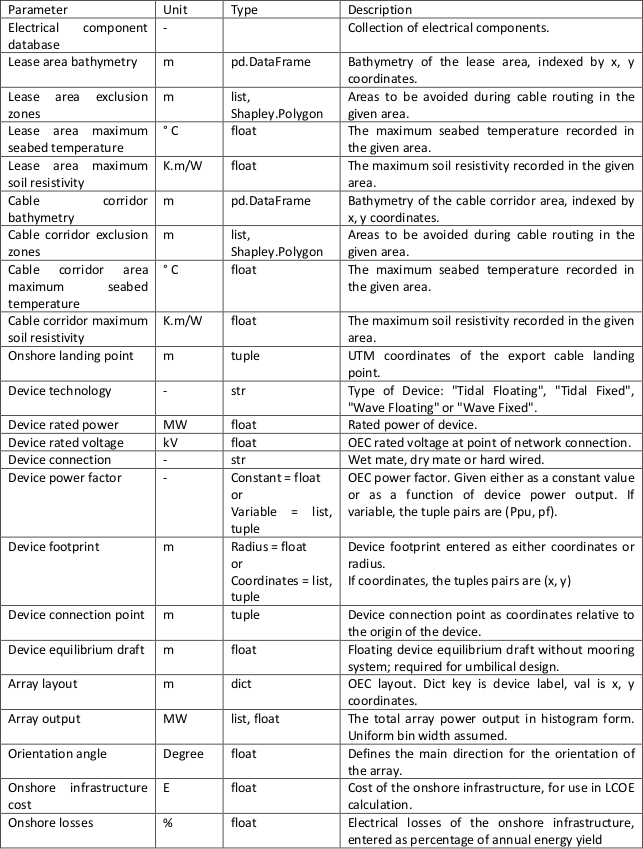
Fig. 7.46 Inputs

Some users options available to constrain the solution are shown in Fig. 7.47. In this table, the name of the ConfigurationOptions attribute is also included for completeness.

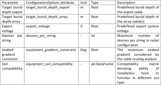
Fig. 7.47 Options

7.2.2.3. Execution¶

The sequence of commands to run the Electrical Sub-Systems moduleis as follows:

>>> electrical_instance = Electrical(site, array, export, options,
database) >>> solution = electrical_instance.run_module(plot = True)

The inputs to Electrical are the classes described in the previous section. The solution returned is an instance of the Network class, which corresponds to the best obtained network.

A basic plot of cable routes and collection point locations is available for display when running outwith the DTOCEAN tool. The visibility of this is controlled by the plot argument of run_module() method.

As part of the global optimisation process, it is necessary to pass control of a number of design variables to the core. This workflow is handled within the core and, if necessary, will constrain certain electrical options in response to the outputs of other modules and overall assessment of array performance (with respect to economic, reliability and environmental thematic indices).

The parameters of influence in the Electrical Sub-Systems module are defined in Table 6.8. In normal execution, these variables form part of the Electrical Sub-Systems module output and should be not constrained; however, they must be defined at the module interface for use in the global optimisation process. Accordingly, these are considered optional, with default None values, and the Electrical Sub-Systems module is designed to check the status and value of these parameters at initiation. It should be noted that this parameter list is not finalised and is subject to further research, both at a local and global optimisation level.

Other parameters which may have an influence on the electrical network, e.g. OEC rated voltage, are already defined as project specific variables. As such, modifying these parameters is considered only as part of the process of creating a new project.

7.2.2.4. Output data¶

As the solution returned by the Electical Sub-Systems modules is an instance of the Network class, specific results can be accessed using the Network object attributes. A printed summary is available by using the print_result() method:

>>> solution.print_result()

The values included in this display are:

Annual Yield: The annual yield at the onshore landing point;
Bill of materials: A summary of the economic data;
Component Data: A table which includes x and y coordinates of all components and quantity/length values. A database reference is included to allow the user to access additional information. The marker can be used in combination with the Hierarchy and Network design data structures to locate the component within the network layout;
Hierarchy: A dictionary structure representing the connections between the different sub-systems. Nested lists are used to denote series and parallel combinations of components/sub-systems: components at the same level are in series with each other and in parallel with components at other levels. The in this structure are the database keys from the Component Data table. This should be read from the array level down;
Network design: Similar to Hierarchy data structure but using component markers to allow identification of specific components;
Cable routes: A summary table of the cable routes;
Collection points: A summary table of the collection point data;
Umbilical cables: A summary table of the umbilical cable designs.

A high level overview of the output data is included in Fig. 7.48, which matches the parameter from the output display with the Network class attribute.

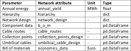
Fig. 7.48 Outputs

7.2.3. Tables of Database Fields¶

Electrical component description tables

Fig. 7.49 Static and dynamic cable component database fields.

Fig. 7.50 Wet and dry-mate connector component database fields.

Fig. 7.51 Transformer component database fields.

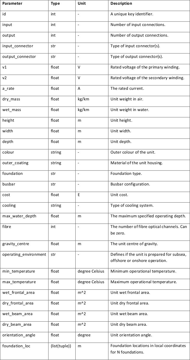
Fig. 7.52 Collection point component database fields.

Fig. 7.53 Switchgear component database fields.

Fig. 7.54 Power quality equipment component database fields.

References

R. Alcorn and D. O’Sullivan, Electrical Design for Ocean Wave and Tidal Energy Systems, vol. 1, London: IET, 2013.

J. Bauer, J. Lysgaard, “The offshore wind farm array cable layout problem: a planar open vehicle routing problem,” J Oper Res Soc (2015) 66: 360

7.3. Moorings and Foundations¶

In this section, the requirements, architecture and functional specification of the Moorings and Foundations module are summarized. For further information the reader is directed towards Deliverable 4.5 (DTOcean, 2015e).

7.3.1. Requirements¶

7.3.1.1. User Requirements¶

The main aim of the DTOcean Moorings and Foundations design module is to perform static and quasi-static analysis to inform or develop mooring and foundation solutions that:

are suitable for a given site, the OEC device (and substation), and expected loading conditions

retain the integrity of the electrical umbilical that connects the OEC device to the subsea cable

are compatible with the array layout (i.e., prevents clashing of neighboring devices) and subsea cable layout

fulfil requirements and/or constraints determined by the user and/or in terms of reliability and/or environ- mental concerns; and

possess the lowest capital cost

By default the module identifies a suitable mooring and foundation configuration based on the supplied characteristics of the site and devices which make up the array. However it is possible for the user to shortcut certain decisions that would be made by the module in order to constrain the design space to a preferred set of pre-selected parameters, such as mooring or foundation type and foundation locations. Furthermore, whilst the database will be preloaded with a set of mooring and foundation components it will be possible for the user to constrain the component selection process to a desired set of components.

7.3.1.2. Software Design Requirements¶

The design of the moorings and foundations design module is outlined in this section. At first, dataflow through the module will be linear, utilizing inputs originating from:

the user (via the graphical user interface or GUI),
the Hydrodynamics and Electrical Sub-Systems modules (umbilical requirements and subsea infrastructure details) and
from the global database. As part of the global design process, all these inputs will be passed to the Moorings and Foundations module through the core. In addition the Moorings and Foundations module also interacts with the Umbilical module. The priority in the first instance will be to select a solution with the lowest capital cost and to pass this (via the core) to the O&M module to determine configuration reliability and LCOE (see economics module section below for more information). The environmental impact of the configuration will also be assessed (see environmental module section for more information), albeit externally to the module.

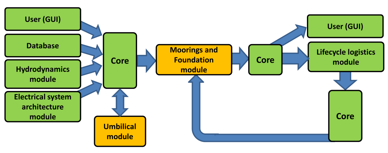
Fig. 7.55 High-level dataflow to and from the Moorings and Foundations module showing constraint feedback

If the solution is not feasible in terms of its economic, reliability or environmental impact metrics or logistical feasibility, an alternative mooring or foundation solution will be sought by initializing a subsequent run of the DTOcean software. Subsequent runs of the Moorings and Foundations module will be constrained by feedback provided by the O&M module and the environmental impact algorithms (e.g. setting a reliability constraint so that only components with reliabilities above a certain threshold can be selected).

The Moorings and Foundations module comprises four interlinked sub-modules including: the System and environmental loads sub-module, Substation sub-module, Mooring sub-module and Foundation sub-module. In addition the Mooring sub-module communicates with the Umbilical module located outside of the Moorings and Foundations module (with communication occurring via the core). The class of the Umbilical module is described below. The figure below shows the general dataflow between these sub-modules. The module operates on a device-by-device basis until all of the devices within the array have been analyzed.

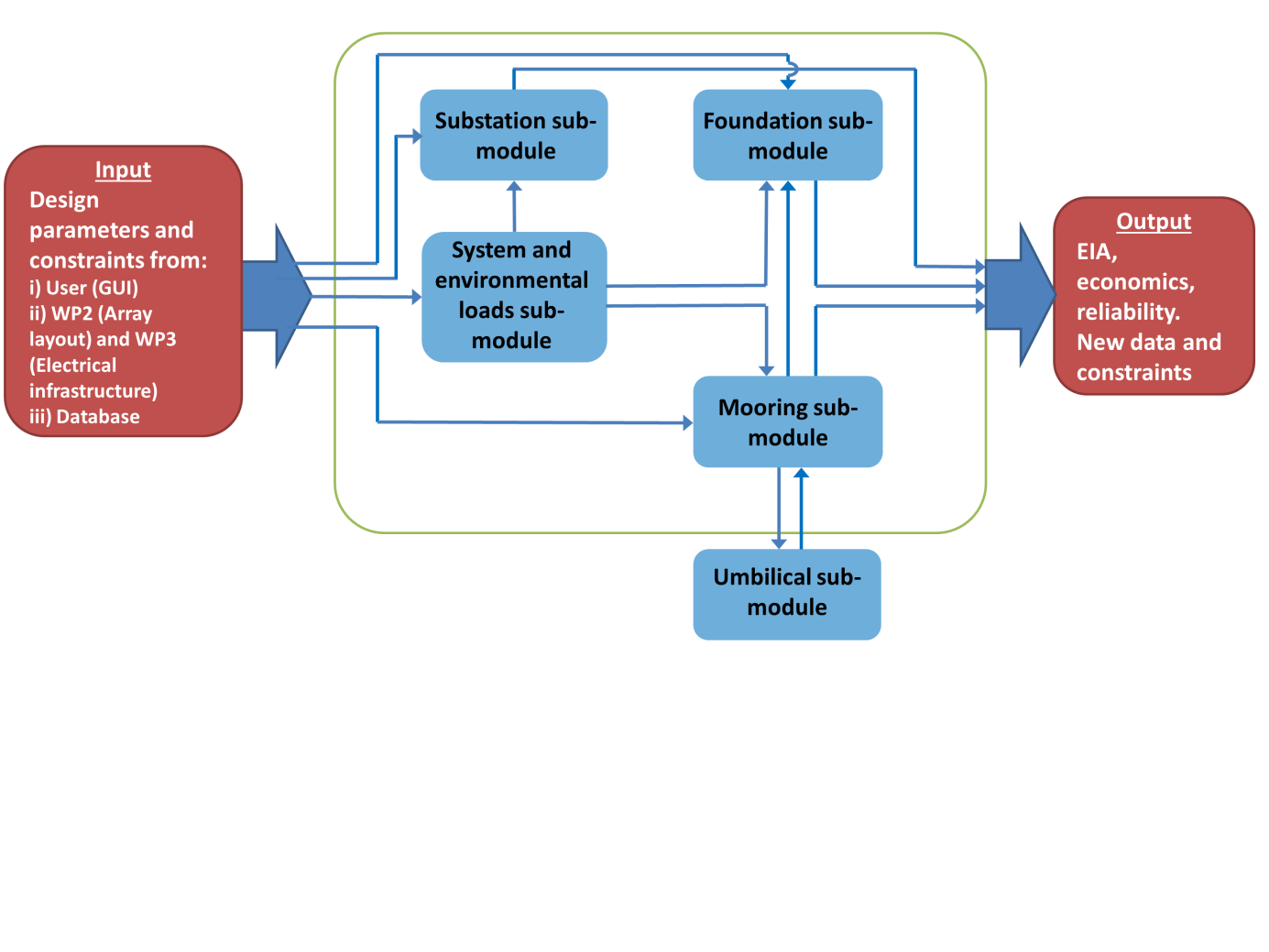
../_images/dataflow_external_moorings.png

Fig. 7.56 High-level dataflow within and external to the Moorings and Foundations module

The calculation procedure invoked within the Moorings and Foundations module will depend on whether the system is floating or fixed. Floating systems require a mooring system and anchors to keep the system on station. It can be seen in the dataflow graphic that dataflow occurs between the Mooring sub-module and Foundation sub-module to allow suitable anchors to be selected. Fixed systems require a foundation to provide a permanent connection between the system support structure and seafloor. Both fixed and floating systems require an umbilical, whilst an array may require a substation. The type of system is therefore a specific input defined by the user and hence determines which of the sub-modules within the Moorings and Foundations module will be used (e.g. in the case of a fixed system the mooring sub-module is redundant and therefore not used).

Each potential design within the Moorings and Foundations module is assessed in order to make an informed decision regarding its suitability. Several standardized design approaches have been adopted for this, drawing from certification guidance, recommended practices and published literature (e.g. (Det Norske Veritas, 2010; Det Norske Veritas, 1992; Det Norske Veritas, 2013a; Det Norske Veritas, 2013b; Bureau Veritas, 2015; Health and Safety Executive, 2001), see also Fig. 7.57). Further discussion of limit states used in mooring and foundation design and the applicability of existing standards can be found in Deliverable 4.5 (DTOcean, 2015e).

Fig. 7.57 Guidance documentation used to develop the Moorings and Foundations module

The external Python libraries employed by the Moorings and Foundations module are as follows:

numpy
pandas
scipy

7.3.2. Architecture¶

7.3.2.1. Overview¶

The Moorings and Foundations module comprises two main Python modules. MoorFound_Main.py acts as an interface between the user or core and the module and also calls the classes within the Moorings and Foundations module. MoorFound_Core.py comprises the classes and functions required to carry out design and analysis of the Moorings and Foundations sub-system. As can be seen from the following figure with MoorFound_Core.py there is interaction between the classes within the Loads, Moor, Subst and Found classes. These processes are summarized in the module processes table.

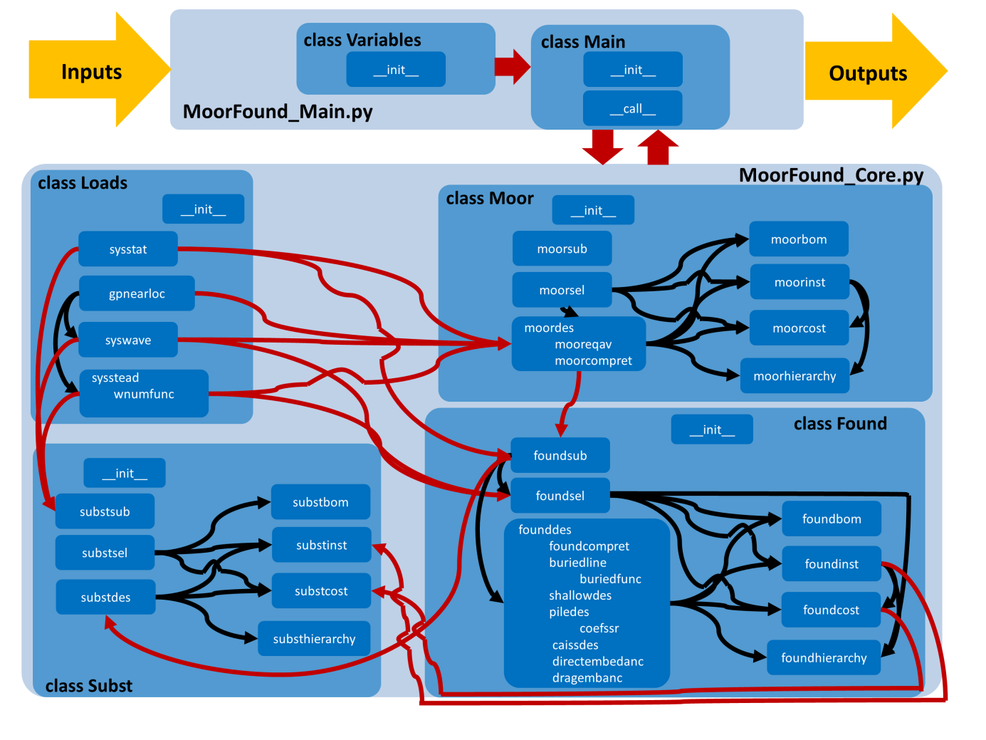
Fig. 7.58 Interaction between the various classes and functions of the Moorings and Foundations module

Fig. 7.59 Summary of internal Moorings and Foundations module processes

7.3.2.2. Dataflow between the functions¶

Dataflow between the internal Moorings and Foundations functions is shown in detail in the above figure. A discussion of the submodules within the Mooring and Foundation module is provided in the following subsections.

All calculations performed within the Moorings and Foundations module are associated to a Device ID number (e.g. device0001) which is utilized by all of the modules within the software. The Main class within Moor- Found_Main.py has a global for loop to sequentially analyze each device, starting at device0001 and ending at deviceN.

7.3.2.3. Loads class¶

The global position of the device (from the Hydrodynamics module), site parameters (i.e. bathymetry and tidal range), in addition to the system properties (i.e. mass, centre of gravity and geometry) as specified by the user, are used to determine the static loads experienced by the device and any eccentric loading. These results are utilised by the Moor and Found classes. For the Subst class the same static, steady and wave calculations are carried out for the substation using information provided by the user or Electrical Sub-Systems module.

Calculation of the design loads is carried out according to the general methodology outlined in (Det Norske Veritas, 2013b) and (Det Norske Veritas, 2011) (Det Norske Veritas, 2011). Two simplified geometries are considered by the Moorings and Foundations module for devices and support structures; cuboids and vertical cylinders. If the device is a tidal turbine, the thrust experienced by the support structure is estimated based on the prescribed surface current, the rotor swept area, hub height and either a thrust coefficient or the maximum value of the user-supplied thrust curve. By default, a 1/7 power law depth distribution is used. This result contributes to the calculation of steady loads on the system.

Static loads are calculated in the sysstat function. In the sysstead function the specified wind and wave conditions3 in addition to current are used to estimate the steady loads on the system. These calculations utilise drag and inertia coefficients stored in the database4 as well as the user-specified wet and dry frontal areas. Mean drift loads are estimated using appropriate analytical approaches.

The next stage is the syswave function, which for floating devices is used by the Moor class to estimate displacement of the device about the mean offset position. The approach used to calculate wave loads on the device or structure depends on whether diffraction is important, and this is judged by the size of the structure in relation to the incident wave parameters and water depth at the device location. If diffraction should be considered, hydrodynamic parameters calculated by the Hydrodynamics module, including added mass, radiation damping and first- order wave load RAOs are used (if available for the translation mode being analysed. If the diffraction regime is not relevant, wave loads on the structure are estimated using the Morison equation and the aforementioned drag and inertia coefficients. Slow drift wave forces are also estimated using the approach given in Chakrabarti (Chakrabarti, 2005).

7.3.2.4. Moor class¶

If the device is floating, mooring systems with anchors are considered. The user may have a particular mooring system type in mind, perhaps from laboratory experiments or field trials of a single device.

If the location of the anchors or a maximum footprint radius has been specified by the user then these values are used in the definition of the mooring system geometry. Alternatively, an anchor radius is set by the Moor class using a relationship between the mooring line length and water depth (Fitzgerald & Bergdahl, 2007), based on the supplied site bathymetry as well as maximum and minimum water level values.

The moorsel function determines if a catenary or taut moored system is most suitable for the application, based on the maximum tidal range of the site and whether the device must remain at the same specified level in the water column throughout all states of tide.

The moordes function first considers a mooring system comprising chain only using the user-supplied fairlead locations. The umbilical will be included in the analysis as an additional line. For comparative purposes chain- synthetic rope configurations will also be considered. The selection of components which make up each configuration will be based on connecting sizes accessed from the database to prevent incompatible components from being selected.

The first calculation step determines the static equilibrium and pretension of the lines without the device in place. The geometry in combination with the static system loads calculated by the Loads class is used to determine the equilibrium position and mooring system tensions. The moorcompret function is used to generate an initial mooring system configuration. If the mooring line tensions exceed any of the component minimum break loads (with a factor of safety applied) alternative components are sought. The moorcompret function also ensures that connecting components are compatible by only selecting components of the same nominal size from the database.

Once static equilibrium has been achieved, the steady wind, current and mean drift loads calculated in the Loads class are used to determine the new equilibrium position and line tensions. A check is made to ensure that the calculated horizontal offset (surge/sway) is within the maximum displacement amplitude limits set by the user and compatible with the specified array layout. Again if the configuration is unsuitable in terms of line tensions, alternative components will be sought from the database function. Two main calculation steps are carried out by the moordes function, corresponding to Ultimate Limit State (ULS) and Accidental Limit State (ALS) analyses. The line with the highest tension calculated in the ULS run is removed for ALS analysis.

The quasi-static calculations performed by mooreqav are inherently simple and do not consider the dynamic behaviour of the mooring lines. Therefore a fully coupled dynamic calculation is not carried out by the module. Instead the module provides a first approximation to mooring system loads and configuration suitability by approximating the (quasi-static) limits of motion and mooring tensions due to a first-order wave excitation and second-order wave drift forces. The criteria which will be used to determine the suitability of the mooring configuration are listed in Deliverable 4.5 (DTOcean, 2015e). The Moor class includes an iterative scheme to specify alternative mooring components if the mooring configuration is unsuitable.

7.3.2.5. Found class¶

If the device is fixed, foundations instead of anchors are considered. The user may have a particular foundation type in mind in order for the foundation to be compatible with the support structure and in this case the decision tree in the foundsel function is not used. For a fixed system it will be necessary for the user to specify the location of the foundation points with respect to the local system origin and orientation.

The foundation type decision tree uses site information (i.e. bathymetry, soil type, soil depth and layering) specified by the user as well as accessing the database for available foundation and anchor components to determine the most suitable range of foundation or anchor technologies. The decision tree comprises a number of matrices to aid the selection process and exclude unsuitable technologies (for further details see Deliverable 4.5 (DTOcean, 2015e)).

In the case of a moored device, anchor positions and maximum load vectors are used to determine suitable anchoring systems, which are determined based on soil type, soil depth and layering in addition to load direction (with the latter originating from the Moor class). If shared anchoring points are deemed to be feasible by the Moor class then this will also limit the selection of anchor types to those which are compatible with multi-directional loads. For fixed structures, soil type (including depth and layering) is the main deciding factor. Soil heterogeneity across the site could result in several different foundation or anchor solutions. For an array of devices a large selection of foundation or anchor types will not be practical nor economically viable, and hence the free selection will probably have to be constrained as part of the global optimization process, particularly for large footprint, spread mooring systems.

Within the founddes function each foundation type has its own calculation procedure. Most approaches involve first determining the applied loads, applying safety factors and then based on the supplied soil parameters, the size and/or penetration depth of the foundation are adjusted iteratively to suit the application. Basic structural (stress) analysis is only conducted for pile foundations.

7.3.2.6. Subst class¶

This operates in a similar way to the Found class, albeit it considers only pile foundations (i.e. monopiles for above-water substations gravity foundations for substations mounted directly on the seafloor). The location and features of the substation are determined by the Electrical Sub-Systems module, with static, steady and wave induced loads calculated within the Loads class. To avoid repetition of code the Subst class calls the same functions used for device analysis.

7.3.2.7. Umbilical module¶

Within the external Umbilical module the umbilical geometry is defined based on the location of the subsea cable (as specified by the Electrical Sub-Systems module) and required umbilical properties and the bathymetry of the site (stored within the database). The equilibrium geometry of the umbilical is determined iteratively. Two options are available depending on whether the device is fixed (a ‘hang-off’-type geometry from the subsea cable up to the J-tube) (Det Norske Veritas, 2014) or floating (‘Lazy-wave’ geometry) (Ruan, Bai, & Cheng, 2014).

The calculated geometry and umbilical constraints (minimum break load and minimum bend radius) are used by the Moor and Found classes.

7.3.3. Functional Specification¶

User interaction with the Moorings and Foundations module is described within this section.

7.3.3.1. Summary of the modelling approach¶

By default the module operates in an optimised mode based on the user-supplied site and device parameters. It is possible for the user to manually constrain the design space by specifying certain parameters (e.g. the pre-selectable foundation and mooring system technology parameters: prefound and premoor)

At first, the solution with the lowest capital cost is identified and passed on to the other modules

A similar approach to mooring (floating devices) or foundation (fixed devices) design is used for WECs and TECs

Only static and quasi-static analyses are conducted by the module

Only catenary or taut moored configurations are modelled for floating systems

Only load cases for ULS and ALS are considered

With the exception of pile foundations, structural analysis of foundations or anchors is not carried out and instead these components are assumed to be rigid. The focus of the Found class is instead the interaction between the foundation or anchor and soil for lateral and axial load analysis

The user will be able to select a series of safety factors based on their preference and/or the requirements of the relevant certification agency (i.e. API, DNV, IEC etc.)

Within the limits of the module the identified solution will be, in quasi-static terms, fit-for-purpose for the application. Using the configuration output data, the user will then be able to carry out dynamic systems analysis to confirm configuration suitability using external third-party software

7.3.3.2. Warnings¶

The moorings and foundations module will output warning messages to the user in situations where either the tool is unable to successfully produce a solution or where the tool is making assumptions that the user needs to be aware of. In the case that the tool is unable to produce a solution then the warning message will assist the user in locating where the issue lies and which input parameters need to be adjusted. A list of the warning messages is included below:

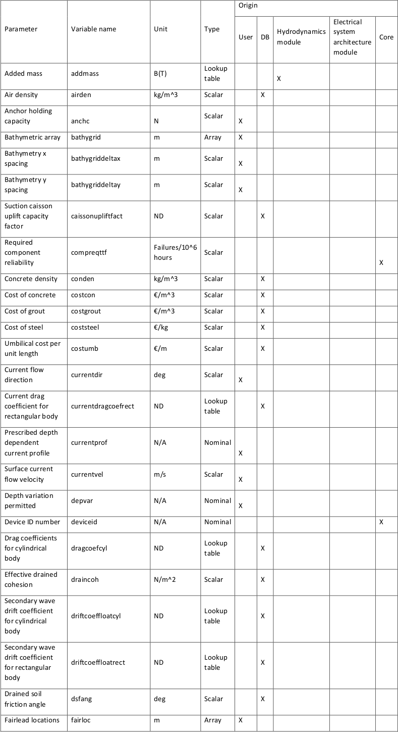
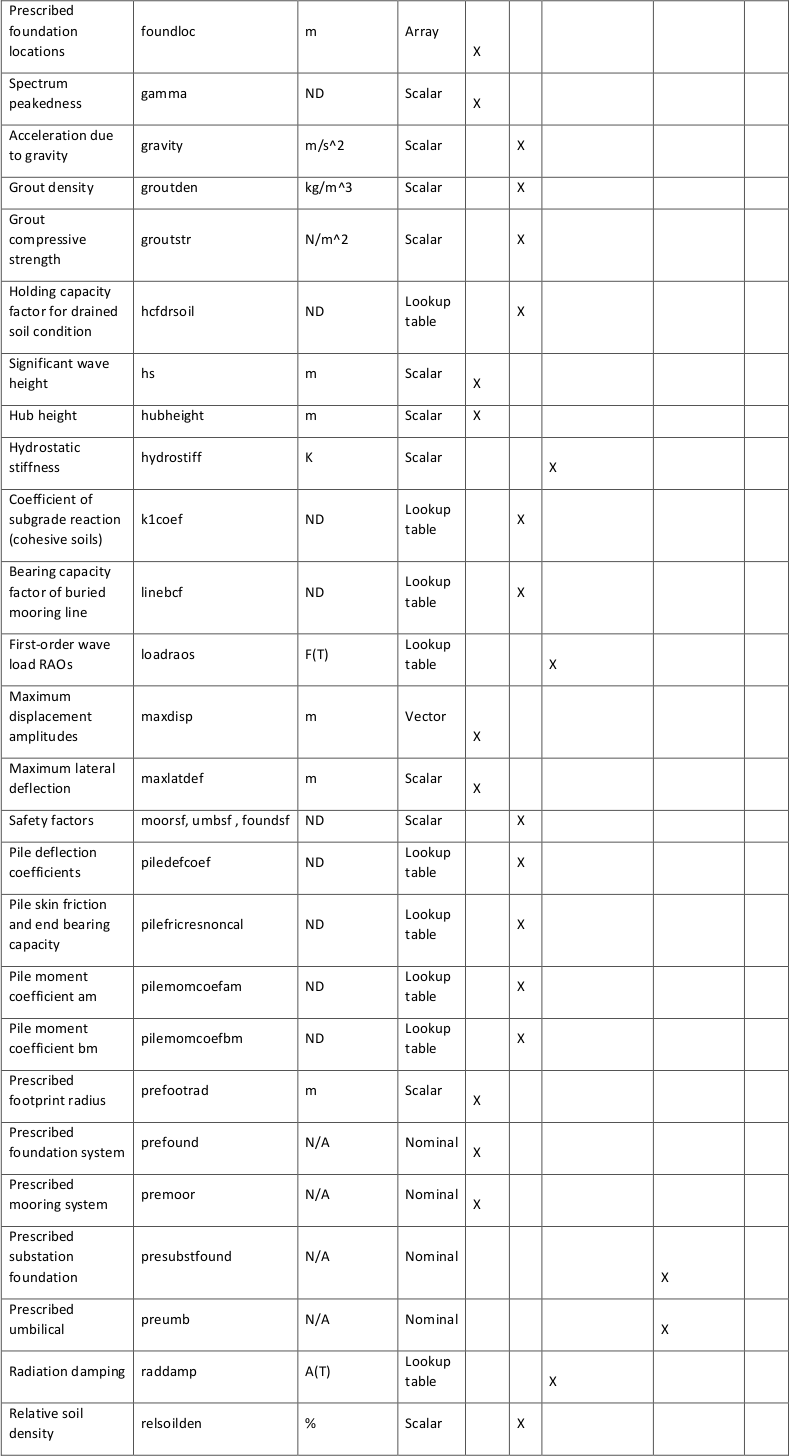
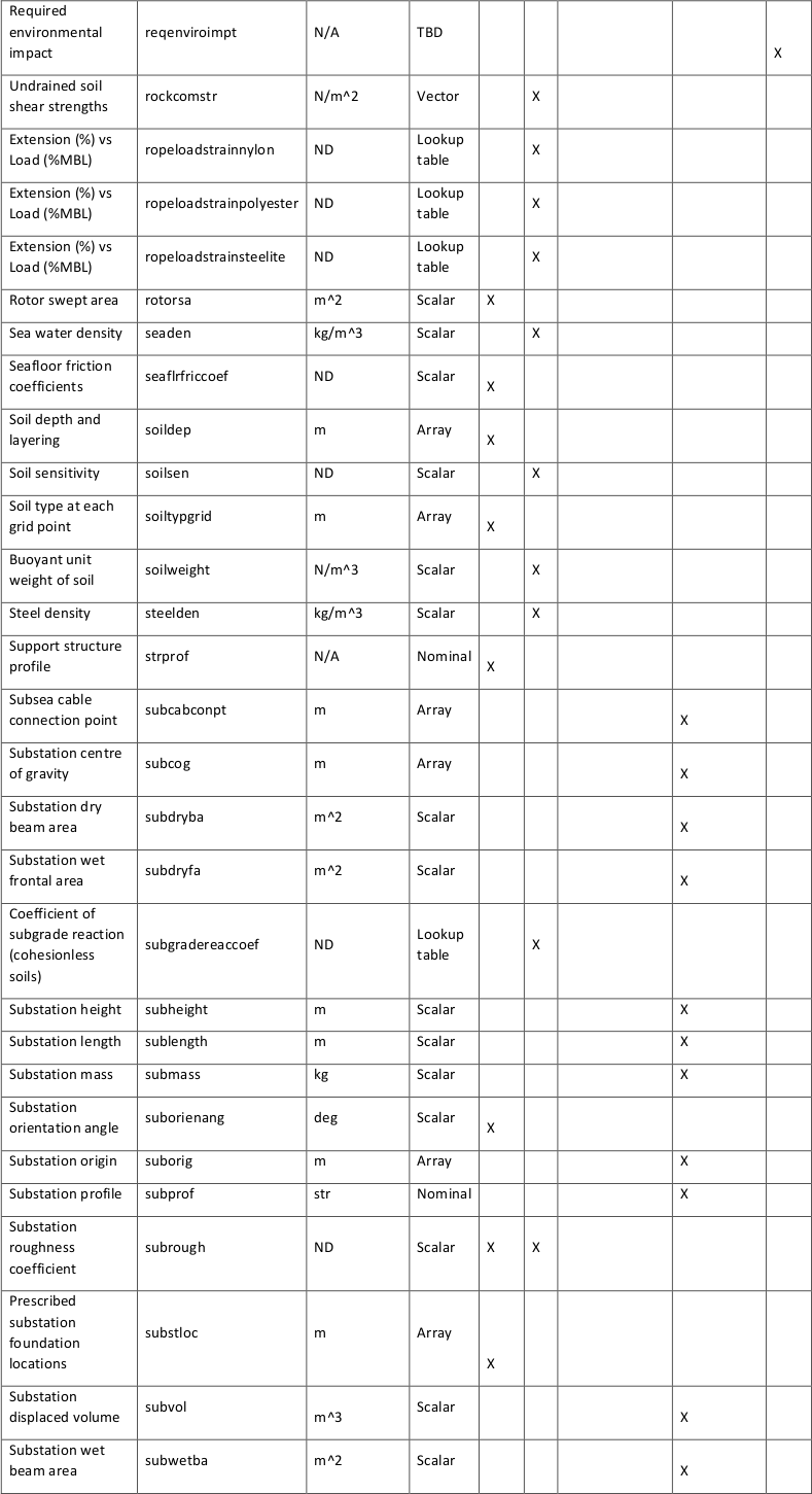
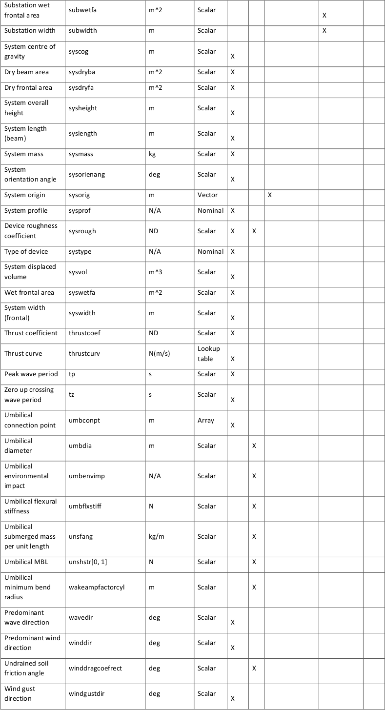
7.3.3.3. Inputs¶

The following table gives a comprehensive list of all inputs required by the moorings and foundations module:

7.3.3.4. Outputs¶

The mooring and foundation solution is details in a number of tables. To elucidate further, the Moor, Found and Subst classes all output the following variables:

Configuration hierarchy

Nested list comprising main component names for the mooring and foundation systems. This is used by the Reliability Assessment sub-module.

Configuration bill of materials

Bill of materials in dictionary format comprising mooring and foundation elements for N foundation/anchor points:

foundation type (str) [-],

foundation subtype (str) [-],

dimensions (list):

width (float) [m],

length (float) [m],

height (float) [m],

cost (float) [euros],

total weight (float) [kg],

quantity (int) [-]

grout type (str) [-],

grout volume (float) [m3],

component identification numbers (list) [-]

Configuration installation parameters (including key seafloor parameters at installation locations) in pandas table format for N foundation/anchor points:

device number (int) [-],

foundation number (int) [-],

foundation type (str) [-]’,

foundation subtype (str) [-],

x coord (float) [-],

y coord (float) [-],

length (float) [m],

width (float) [m],

height (float) [m],

installation depth (float) [m],

dry mass (float) [kg],

grout type [-],

grout volume (float) [m3]

cost (float) [euros],

total weight (float) [kg],

quantity (int) [-]

grout type (str) [-],

grout volume (float) [m3],

component identification numbers (list) [-]

Configuration installation parameters (including key seafloor parameters at installation locations) in pandas table format for N foundation/anchor points:

device number (int) [-],

foundation number (int) [-],

foundation type (str) [-]’,

foundation subtype (str) [-],

x coord (float) [-],

y coord (float) [-],

length (float) [m],

width (float) [m],

height (float) [m],

installation depth (float) [m],

dry mass (float) [kg],

grout type [-],

grout volume (float) [m3]

7.3.3.5. Calculation time¶

Calculation times are dependent on the system in question. Indicative values for one device are provided in Fig. 7.60.

Fig. 7.60 Indicative calculation times for a single device subjected to several wave conditions

7.4. Installation¶

As any other computational module, the Installation module aims to solve a given physical problem and return the required outputs. However, unlike the upstream computational modules, no physical array sub-component is selected nor designed as part of the BoM. In contrast, the Installation module provides optimal logistic solutions by selecting feasible vessels, ports and equipment to accomplish the installation phase. The optimal logistic solutions are those minimising the overall cost of each logistic phase.

7.4.1. Requirements¶

7.4.1.1. User Requirements¶

The Installation module seeks to minimise the cost of installing all components/sub-systems chosen by the three upstream computational modules (i.e. Hydrodynamics, the Electrical Sub-Systems and Moorings and Foundations). In other words, the Installation module covers the following elements:

Installation of wave or tidal devices; as positioned by the Hydrodynamics module
Installation of the electrical infrastructure components; as designed by the Electrical Sub-Systems module
Installation of the moorings & foundations; as designed by the Moorings and Foundations module

There are nine logistic phases under consideration which cover the OEC device and the entire BoM as compiled by upstream computational modules, as listed below:

Installation of OEC devices
Installation of driven pile foundations
Installation of gravity based structures
Installation of mooring systems
Installation of static export power cables
Installation of static inter-array power cables
Installation of dynamic power cables
Installation of offshore collection points
Installation of cable external protection

It should be noted that if the user wishes to use the Installation module to assess the installation of only a restricted part of the entire BoM (comprising devices, moorings & foundations and the electrical infrastructure), then the quantity of the item to be ignored by the Installation module should be set to “None”. For example, this allows the user to evaluate only the installation of the devices while disregarding the installation of the other components. In this mode of operation, the commissioning date will be given as the moment when all the components required to be installed, have been completed. There is no estimation of the duration of installation phases that have not been requested for simulation.

7.4.1.2. Software Design Requirements¶

As for the logistic functions, details of the algorithms embedded in the Installation module can be found in Deliverable 5.6 (DTOcean, 2015h). Only minor features extend the logistic functions to form the Installation module, which are:

an installation procedure definition sub-module
the selection of the base installation port corresponding to the port from which all marine operations necessary to complete the installation phase will be departing from and
an optimisation routine to find the most economically attractive logistic solution to carry out all steps of the installation phase

7.4.2. Architecture¶

The working principle of the Installation module progresses from the collection of all inputs until the generation of the formatted outputs.

In summary, the Installation module comprises the following components:

An external logistic phase sub-module: this is where the operation sequences and vessels & equipment combinations are defined for all logistic phases
An installation procedure definition sub-module which is divided into two functions;
- One defining the scheduling rules to determine the sequence of the logistic phases; this function makes use of default “Gant chart” rules to establish the relationship between logistic phases in terms of requirements to have some components of the bill of material already installed prior to install another one. For instance, this function assumes by default that the OECs must always be installed only once the entire electrical infrastructure and the moorings/foundations have been deployed at site
- Another function selecting the base installation port; the selection of the base installation port follows a twofold sequence. First, only ports having at least one quay that can accommodate the largest item from the bill of material are kept (it is also verified that the port possesses a dry dock if it is a requirement for the device assembly/load out). Secondly, the nearest port to the centre of the lease area specified by the user is selected
Logistic functions assessment sub-module: it contains the core assessment of all marine operations required to complete the installation phase and must complete two roles:
- The selection of suitable maritime infrastructure: characterises the logistic requirements associated with the port, vessel(s) and equipment for each logistic phase and subsequently filters out only the technically feasible solutions
- The performance assessment of logistic phases: performs the assessment of each logistic phase respectively in terms of time scheduling, cost, environmental impact and risk value
An optimisation routine: the most inexpensive feasible logistic solution is chosen for each logistic phase. Ultimately, the combination of the optimal solutions for each logistic phase forms the overall optimal installation phase solution

The optimisation routine internal to the Installation module simply consists of isolating the feasible logistic solutions which returned the minimum total cost for a given logistic phase \(C_{lp}\). At the end of the Installation module, the outputs are sorted and formatted in the most convenient way for future results presentations. Full details of the calculation of \(C_{lp}\) can be found in (DTOcean, 2015h). Furthermore, the default values tables are also available in the same deliverable.

7.4.2.1. Logistic Functions¶

The purpose of the logistic functions is to provide both the Installation module and the Operations and Maintenance module with the means to evaluate marine operations that are called “logistic phases”. For each logistic phase, a common set of logistic functions are designed. These logistic functions consist of:

Defining the default operation sequences (breakdown of the logistic phase into individual task starting from mobilisation until demobilisation) as well as defining the default vessel(s) & equipment combinations that can carry out the logistic phase

Characterizing the logistic requirements in terms of port, vessel(s) and equipment

Selecting technically and physically feasible solutions of port/vessel(s)/equipment

Assessing the performance of these feasible solutions in terms of:

Schedule (or time efficiency)

Cost

Environmental impact

It is not expected for the calling computational modules to define the default operation sequences and vessel(s) & equipment combinations, thus the first scientific operations underlying the logistic functions is the characterization of the logistic requirements and subsequent selection of the feasible maritime infrastructure. This process is governed by the “feasibility functions”. For each logistic phase, a set of dedicated feasibility functions, responding to the specific characteristics of the logistic operations to be conducted, are defined. It should be noted that a large number of feasibility functions are shared across logistic phases.

Table 6.14 below exemplifies how such feasibility functions are implemented for the port, vessel and equipment, respectively.

In essence, the feasibility functions consist of Boolean operations and inequalities relating array design inputs (typically provided by the end-user or computed by upstream computational modules) to parameters of the mar- itime infrastructure database (ports, vessels and equipment).

In this manual, the comprehensive list of all feasibility functions will not be depicted. For further information, the reader is invited to refer to Deliverable 5.4 for the Installation module (DTOcean, 2015f) and Deliverable 6.5 for the O&M module (DTOcean, 2015g).

Nevertheless, for illustration the tables below exemplify how such feasibility functions are implemented for the port, vessel and equipment, respectively.

In essence, the feasibility functions consist of Boolean operations and inequalities relating array design inputs (typically provided by the end-user or computed by upstream computational modules) to parameters of the maritime infrastructure database (ports, vessels and equipment).

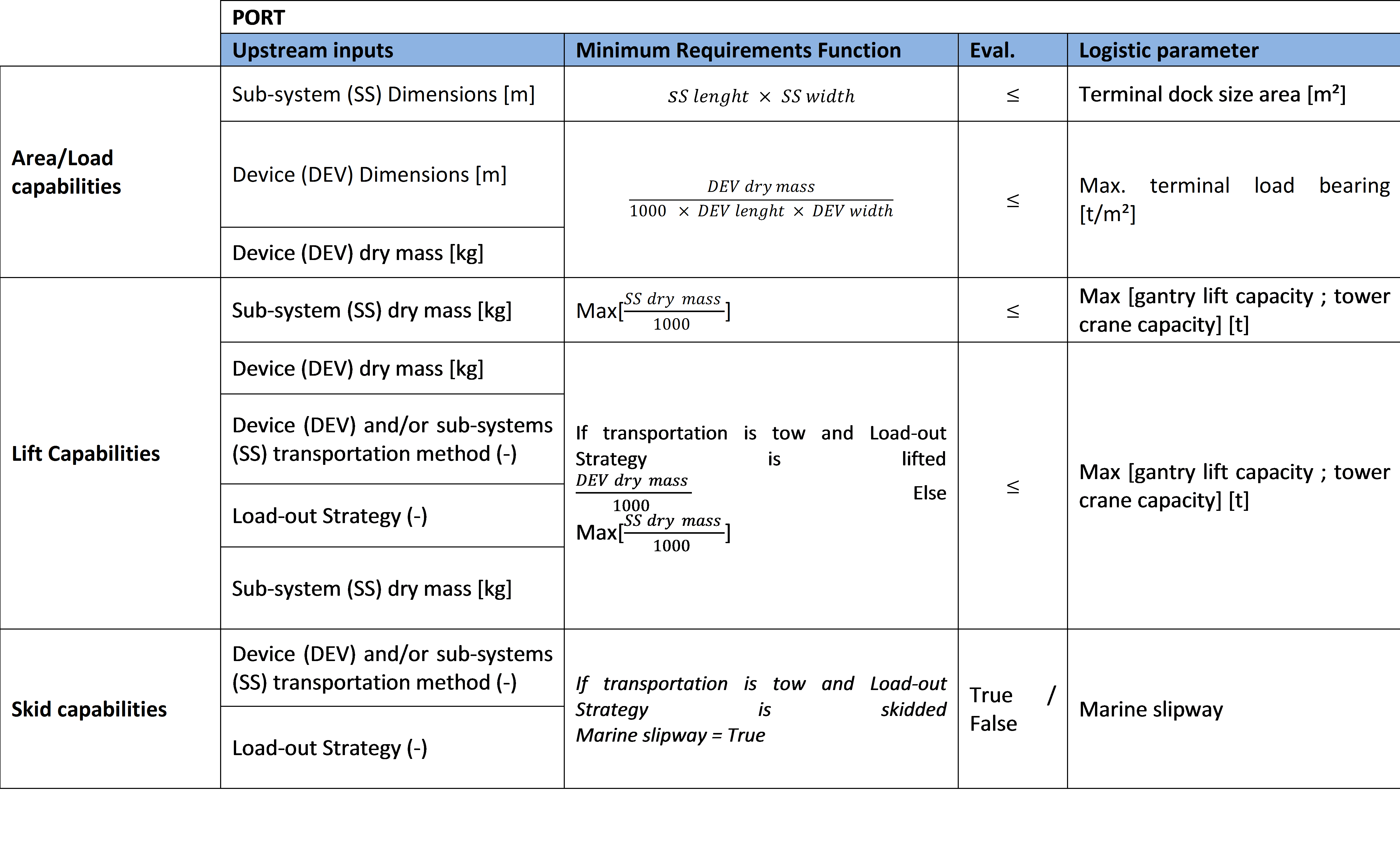
Fig. 7.61 Port feasibility functions during the installation of wave or tidal energy devices

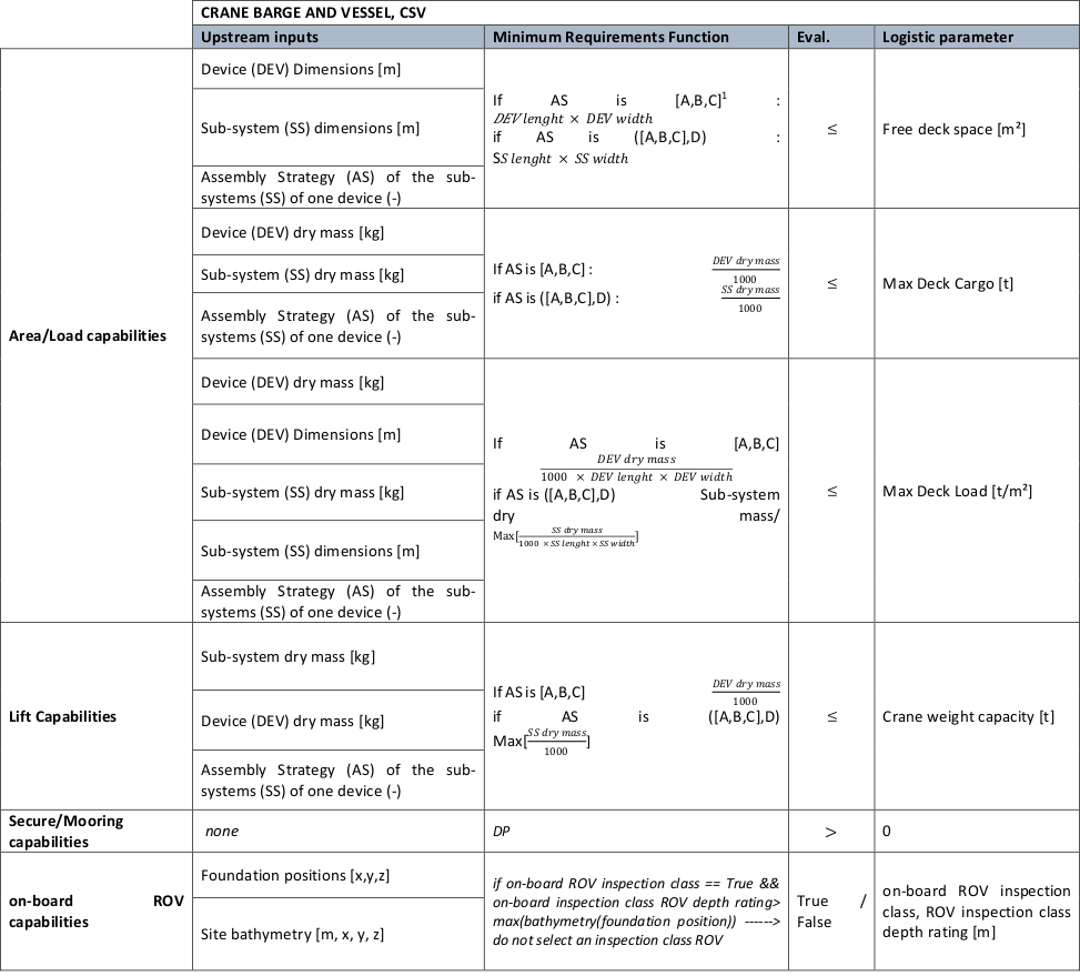
Fig. 7.62 Crane barge or vessel feasibility functions for the installation of wave or tidal energy devices

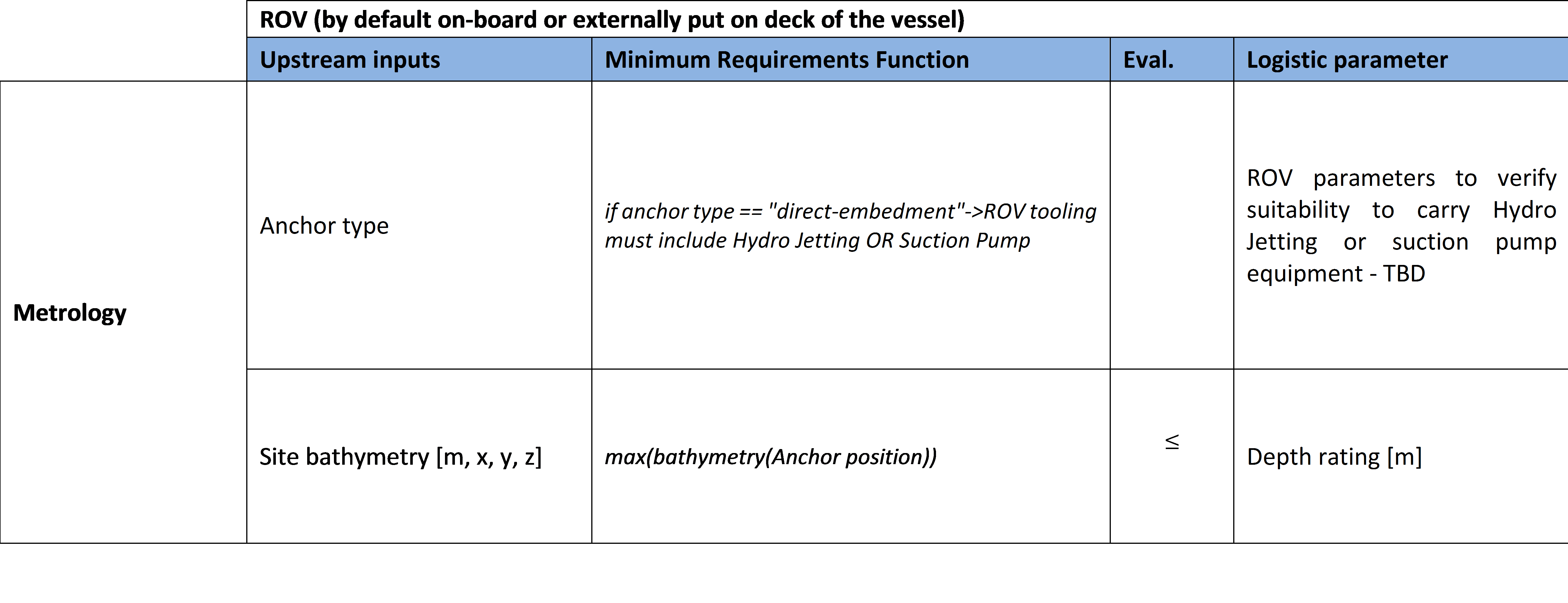
Fig. 7.63 ROV feasibility functions for the installation of a mooring system

A subset of feasibility functions are also defined in order to ensure the compatibility of the port/vessel(s)/equipment combinations. These functions are also inequalities and Boolean operations which essentially verify that the vessel(s) can be accommodated by the port and that the equipment will fit in the corresponding vessel(s).

In addition to the feasibility functions, there exists a second category of algorithms which are named the “performance functions”. Once technically and physically suitable combinations of port/vessel(s)/equipment have been identified, the purpose of the performance functions to discriminate between them based on performance.

The first executed performance function provides a time duration estimate of the logistic phase, denoted \(T_{lp}\). The total time \(T_{lp}\) is the sum of the time spend at port \(T_{port}\), the waiting time for a satisfactory weather window \(T_{wind}\) and the time spent at sea \(T_{sea}\), as summarised in (9) below:

\[T_{lp} = T_{port} + T_{wait} + T_{sea}\]

To access the details of how each element introduced in (9) is calculated, the reader is encouraged to read through the section about the “scheduling functions” in Deliverable 5.6 (DTOcean, 2015h).

The second performance function concerns the cost estimation. In its generic form, the cost of a logistic phase \(C_{lp}\) simply aggregates the port charges \(C_{port}\) and the expenses due to the marine operations \(C_{sea}\). This can be expressed as shown in (10):

\[C_{lp} = C_{port} + C_{sea}\]

A description of each element of (10) can be found in Deliverable 5.6 (DTOcean, 2015h). It also details the requirements for the environmental functions, the last item of the performance functions. Five environmental impacts are assessed by the logistic functions, the results of which are delivered to the environmental impact assessment thematic algorithm.

The logistic functions are required to:

Define the logistic phase in terms of operation sequencing and default vessel(s) & equipment combinations
Characterise the logistic requirements (first step of the feasibility functions)
Select suitable maritime infrastructure (second step of the feasibility functions)
Conduct a performance assessment of all feasible logistic solutions in terms of time efficiency, cost and environmental impact

The inputs, outputs and internal dataflow of the logistic functions are schematically represented in Appendix E. On the left side, all “external” inputs, originating from the end-user or generated by upstream computational modules (including the Hydrodynamics, the Electrical sub-system and the Moorings & Foundations modules), are shown. On the right side, the “internal” inputs, accounting for the maritime infrastructure database and default values, are placed. Unlike “external” inputs, “internal” inputs are established by the developers of the logistic functions and the Installation module, i.e. they will not be exposed to the user.

In addition to the external inputs, there are a number of “internal” inputs within the logistic functions. The maritime infrastructure is a core object that must be accessed when running the logistic functions. While the comprehensive list of the inputs can be found in Deliverable 5.3, these can be summarised as:

Port database: detailed information about European ports with the following parameter categories:
- General Information (13 parameters)
- Port Terminal Specification (17 parameters)
- Port Cranes, Support, Accessibilities and Certifications (16 parameters)
- Manufacturing Capabilities (8 parameters)
- Economic Assessment (8 parameters)
- Contact Details (4 parameters)
Vessel database: detailed information about each vessel type considered in DTOcean with the following parameter categories:
- General Information (9 parameters)
- Main Dimensions and Technical Capabilities (18 parameters)
- Maximum Operational Working Conditions (8 parameters)
- On-board Equipment Specifications (~34 parameters)
- Economic Assessment (4 parameters)
Equipment database: detailed information about each equipment types considered in DTOcean with the following parameter categories (the number of parameters varies from one equipment type to another):
- Metrology (min. 4 parameters)
- Performance (min. 2 parameters)
- Support Systems (min. 2 parameters)
- Economic Assessment (min. 2 parameters)

Finally, default input values must also be provided to the logistic functions. It is import that the user is aware of these default values and so they should be made available to them prior to using the sub-module or by any module that interfaces with it. Common default values pertaining to logistic phases associated with both the installation and O&M modules include:

Average fixed duration values of individual logistic operations
Safety factors relating to selected feasibility functions
Operational Limit Condition (OLC) values for specific individual logistic operations

Once all inputs are correctly passed into the logistic functions, the evaluation of the feasible logistic solutions and performance assessment will approximately consume between 2 to 10 seconds for a single logistic phase. It should be noted that this rough wall-clock time estimation is based on preliminary test run cases which do not represent the full scope (i.e. not all logistic phases covered in the installation and O&M modules have been tested to-date). The more feasible logistic solutions (i.e. the number of suitable combinations of port/vessel(s)/equipment) and the more OLC, the more time is required for the logistic functions to run for a given logistic phase. Finally, it should be noted that this computational time estimate excludes the estimate of the time spent at sea.

The outputs of the logistic functions are:

The list of all logistic requirements associated with the logistic phase
The selected suitable combinations of port/vessel(s)/equipment associated with the logistic phase
The schedule assessment (including the total time \(T_{lp}\)) of each feasible logistic solution associated with the logistic phase
The cost assessment (including the total cost \(C_{lp}\)) of each feasible logistic solution associated with the logistic phase
The environmental impact assessment (including the final score of the five environmental functions concerned with the logistic functions) of each feasible logistic solution associated with the logistic phase

These outputs are assembled in a dictionary with the characteristics shown in the next table.

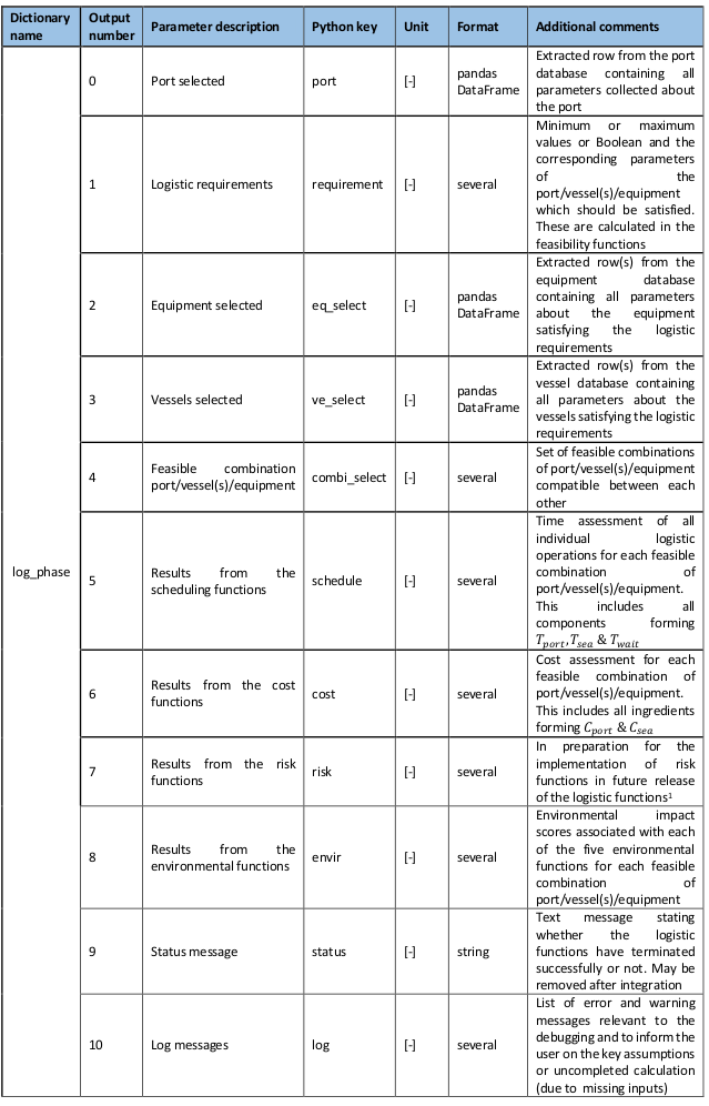
Fig. 7.64 Output dictionary of the logistic functions

7.4.3. Functional Specification¶

In essence, the list of inputs for the Installation module is the same as the one for the logistic functions provided before with only three additional pandas DataFrame tables:

Vertical penetration rates for all piling equipment in all soil types considered in the scope of the DTOcean project
Horizontal progress rates for all cable trenching/laying equipment in all soil types considered in the scope of the DTOcean project
Default Gantt chart rules for the installation planning

Similar to the logistic functions, the main effort to get the Installation module running resides in the preparation of the numerous inputs. Further to the four pandas DataFrames (‘site’, ‘metocean’, ’device’, ‘sub_device’ as depicted in Appendix F) the user must enter, it is also strongly recommended that the user overrides the default values when more accurate data concerning the ocean energy project is available.

Assuming all upstream computational modules have successfully generated the outputs required to feed the Installation module, no intervention from the user is required other than inputting the aforementioned four tables. The Installation module terminates with the formatting of the outputs. Results obtained through the feasibility functions for the nine installation logistic phases convene in a predicted installation plan which contains:

starting and ending dates of all sub-array components installation phases together with the estimated waiting time
selected maritime infrastructure per marine operation
cost breakdown per logistic phase, and
environmental scores per logistic phase

The Installation module returns the dictionary output of the logistic functions presented in Section 6.5.3 for each logistic phase the user wishes to be considered by the Installation module.

7.5. Operations and Maintenance¶

The purpose of the “Operations and Maintenance” (O&M) module is to minimise the impact of the O&M activities on the LCOE. This will be done by calculation / simulation of a cost optimised full operational cycle O&M approach, where different strategies are combined and the actual dates of performance for the individual O&M actions (inspections, maintenance, repair) are optimised with respect to the starting dates and the possibility of parallel scheduling. In an early stage of the DTOcean project, it was decided to perform this optimisation process on a time based approached. Therefore, the module is designed to simulate the full O&M life cycle of an OEC device array by distributing the possible maintenance operations over the entire operational phase (e. g. 25 years) of the array.

The following sections describe the required setup steps and the data to be provided by the user. Furthermore, the implementation of the module with a description of the developed algorithms, the software structure and the definition of the interface for data exchange with other modules (via the core module) is given.

7.5.1. Requirements¶

7.5.1.1. User Requirements¶

The purpose of the O&M module is to simulate the time domain based full life cycle O&M activities of an OEC array. For this purpose, a maintenance plan will be generated for each relevant component as defined by the user. Everything inside the array will be handled as a component, i.e. a component can be:

an infra structure item, e. g. the export cable, the sub-station(s), subsea connectors, switch gear, cable sections in the internal array grid, etc.

an entire device (if no deeper level of detail is required)

components of a device (level of detail will be restricted to the Equimar (Ingram et al., 2011) definition with the four major sub-systems: hydrodynamic converter, PTO, reaction and controller)

The user is can select one of three desired maintenance approaches (“corrective”, “calendar based”, “condition based” (DTOcean, 2014a)) or meaningful combinations of it. The individual maintenance approaches will be further detailed by use of a few parameters, which are described in the following sections. For each component a maintenance plan is generated, and an example can be seen in the Fig. 7.65.

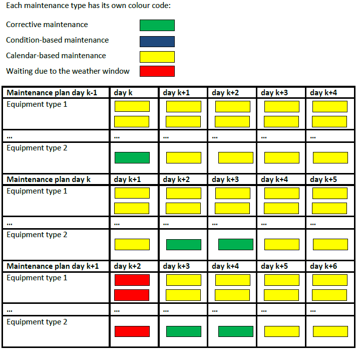
Fig. 7.65 The Schematic overview of a maintenance plan

7.5.1.2. Software Design Requirements¶

The purpose of the O&M module is the modelling of the time domain lifecycle O&M methodology. The O&M module simulates all operation and maintenance activities of the OEC array over its lifetime in the time domain. Costs related to the O&M activities will be calculated and added to the overall LCOE figure. The O&M module can be used to understand and optimise the O&M strategy of OEC array in the planning phase of a project. The minimisation of the maintenance cost will help the decision maker to choose cost-optimal solutions.

Maintenance is defined as the combination of all technical and administrative actions intended to retain an item in, or restore it to, a state in which it can perform its required function (IEEE, 2000). The Fig. 7.66 illustrates a common classification of maintenance strategies, which is based on the standard SS-EN 13306 (SIS Forlag, 2001).

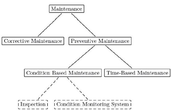
Fig. 7.66 Types of maintenance strategies, partly adapted from (SIS Forlag, 2001).

The maintenance strategies considered in the DTOcean project are defined as:

Corrective maintenance is due to an unexpected failure and is intended to restore an item/component to a state in which it can perform its required function (IEEE, 2000)

Condition-based maintenance is a type of preventive maintenance based on a response to the monitoring information available (SIS Forlag, 2001). It consists of all maintenance strategies involving inspections (noise, visual, etc.) or permanently installed Condition Monitoring Systems (CMS) to decide on the main- tenance actions

Calendar-based (Time-based) maintenance is a type of preventive maintenance carried out in accordance with established intervals of time or number of units independent of any conditioning investigation (SIS Forlag, 2001). It is suitable for failures that are age-related and for which the probability distribution of failure can be established based on fixed time intervals

The O&M costs are known to be an important part of the life cycle OPEX cost of MRE projects. In offshore wind farms, O&M contributes 15-30 % of the total LCOE (Engels et al., 2009). Therefore it is important to develop cost-effective O&M concepts to help MRE projects to be competitive with offshore wind. The optimisation of these concepts addresses the overall resources (personnel and equipment) required to execute the maintenance activities, which inherently include the logistical support.

To model the individual behaviour of components of OEC array devices, the following items need to be considered:

Component annual failure rate

Effect of the failure of the component to other components or devices

The optimised mixture of maintenance strategies to keep the array devices operational

The requirements of the maintenance processes of all components with respect to time/duration, ves- sels/equipment, spare parts and personnel

A typical maintenance process is depicted schematically in the Fig. 7.67 below. All maintenance strategies can be simulated with this process plan. The difference in handling the strategies is mostly setting the time parameters to the respective values. For example, for a calendar/condition based maintenance activity, the “T_Organisation” will be significantly shorter, since the organisational and preparatory tasks (booking of vessels & equipment, mobilising personnel, ordering of spare parts, etc.) can be done before the scheduled operation starts. Another example is a simple inspection, for which the “T_Logistic” can be set to zero because there is no need for ordering spare parts.

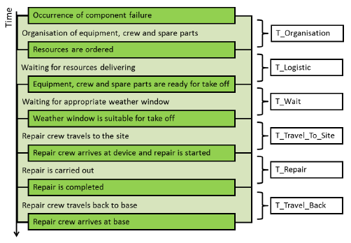
Fig. 7.67 Typical maintenance process

The definition of calendar based maintenance is simply done by setting the interval (e. g. “annual”, “semi-annual”, etc.). Condition based maintenance requires the definition of a “state of health” (SOH) threshold, below which maintenance is mandatory for the component. For this, it is assumed that at the installation / commissioning of an OEC device or after repair / replacement activities, the SOH of a component will be 100%. A linear interpolation simulates the SOH of the considered component. The SOH limit in % that triggers the condition based maintenance is a parameter of the O&M module and will be set by user. The slope of the SOH degradation curve is also defined by the user (see Fig. 7.68).

In time domain simulation the occurrence of a failure has to be estimated over the lifetime of the device. To translate the statistical based failure rates back to the time domain, a Binomial or Poisson process can be used. A Poisson process is a stochastic process that counts the number of events and the time points at which these events occur in a given time interval. The time between each pair of consecutive events has an exponential distribution with parameter λ (intensity) and each of the inter-arrival times is assumed to be independent of other inter-arrival times. Fig. 7.69 depicts an example for the given random parameters.

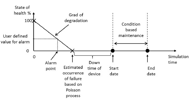
Fig. 7.68 Handling of automated inspection in case of condition-based maintenance

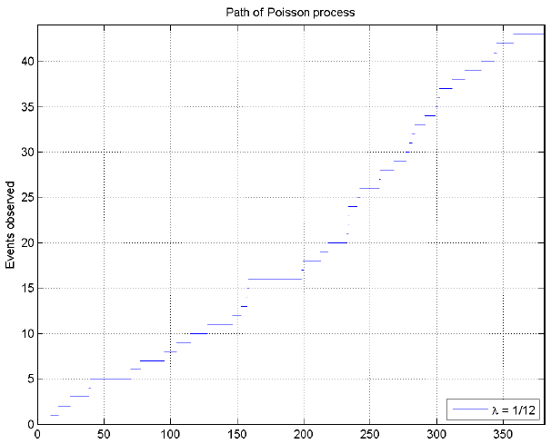
Fig. 7.69 Paths of Poisson process for a 30 year period and a number of 44 events

The optimisation algorithm used to minimise the cost of the O&M for the OEC array has to fulfil the following case:

Optimisation in case of corrective maintenance

Optimisation in case of condition-based maintenance

Optimisation in case of calendar-based maintenance

Optimisation of the interaction between different maintenance strategies (mix strategies)

The user has the option to define different combinations of maintenance strategies. The user may only be interested in the cost optimisation of “unplanned corrective maintenance”, for instance. In this case, no optimisation of mixed maintenance strategy is necessary because the user is required to enforce such a choice. In a second example, the user may be interested in the cost optimisation of a mix of “Unplanned corrective maintenance” and “Calendar- based maintenance” strategy, in which case the module will calculate the optimised solution for the mixed strategy.

Optimisation in case of corrective maintenance

The optimisation approach is based on the clustering of corrective maintenance events with those of the two other strategies considered in scope, i.e. calendar based and condition based. A criterion will be defined by the user as the number of days, which will be the time distance to allow clustering. For example, if a corrective maintenance action is followed by a calendar based maintenance action and/or a foreseeable condition based maintenance action within the next “K” days, the two/three operations will be combined to save costs for logistics (vessel(s) & equipment charges, transportation, etc.). Parameter “K” is user defined.

Optimisation in case of condition-based maintenance

In addition to the above mentioned clustering, the value for the SOH threshold, at which the condition based main- tenance will be triggered, is an optimisation issue. The reason for this is that from a certain SOH on downwards, the power output of an OEC will be reduced (“de-rating”) to extend the remaining life time of the OEC and its components. This will result in less power production and, therefore, reduced energy revenue.

The de-rating process and the condition based maintenance trigger threshold are controlled by user defined pa- rameters. For example, from a SOH value of “X” (in “%”) the power output set point will be reduced linearly from rated power to zero. At a value of “Y” % SOH, the device will be shut down to avoid serious consequential damages. It is 100% > X > Y (Y should be at least 25%).

Optimisation in case of calendar-based

To optimise the calendar based maintenance, either the time interval between two maintenance actions (when a scalar parameter is defined) or the fixed dates for the start of all calendar based maintenance actions during the operational phase can be defined (vector parameter). In principle, a smaller interval for the calendar based main- tenance reduces the probability for the occurrence of device faults and resulting shut downs. On the other hand, it requires more frequent maintenance actions and, therefore, causes higher costs. The parameter for controlling the calendar based maintenance interval is defined by the user. The vector parameter option allows to model individ- ual maintenance approaches/intervals, e. g. the first calendar based maintenance after five years and then every two years.

Optimisation of the interaction between different maintenance strategies (mixed strategies)

In order to handle the interaction between different maintenance strategies (mixed strategies), the following con- cepts are integrated into the optimisation process:

Priority definition of maintenance activities

Priority definition of OEC devices

Time shifting (postponing) of maintenance action on time axis

Parallel shift, number of crew

Priority definition of maintenance activities

Some priorities for maintenance actions will be defined due to the limitation of resources (e.g. vessels, crews). Some examples are:

All maintenance tasks that have already started have highest priority

Corrective maintenance has the highest priority, then condition-based maintenance, and then calendar-based maintenance

Priority definition of OEC devices

A priority parameter controls which device will be repaired first when there is only limited resources or time (weather) windows to perform maintenance activities. For example, if there is a problem with the electrical connection (circuit break) at two OEC devices, the one which is closer to the hub / transformer will be repaired with higher priority since all the following devices in the electrical string will also be affected from the damage. The priority value for an OEC device will be calculated with respect to its position in the electrical string (see Fig. 7.70).

Another item to be considered when calculating the priority is the availability of spare parts. If a spare part for the component to be repaired in device 1 is higher than for another component in device 2, than device 2 will get a higher priority and will be maintained first.

Time shifting

Shifting of a repair action in case of corrective maintenance to the planned calendar based maintenance is an optimisation task and is not trivial. Calendar based maintenance will be done in a defined time section in a year (start and end date are user parameters). For a shifting of the repair action in case of corrective maintenance the device downtime due to the time shifting and, therefore, the revenue losses have to be calculated depending on the position of device in the electrical grid cable string (see Fig. 7.70 and Fig. 7.71). These losses should be compared with the cost advantage of time shifting (e.g. mobilisation cost). The result of this comparison controls if time shifting is required.

Parallel shift, number of crew

Working with parallel shifts means increasing the number of crew required to carry out the work. This results in less time for performing the maintenance action (and, consequently, reduced device downtimes) but will result in higher personnel costs. The optimisation task is to find the minimum LCOE between the loss of energy revenue and the additional personnel costs.

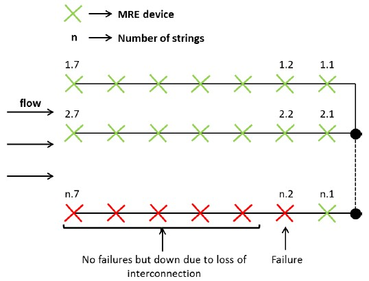
Fig. 7.70 Failure occurrence in n.2 device

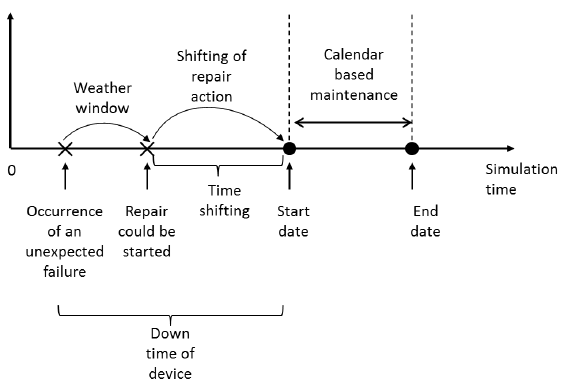
Fig. 7.71 Time shifting of maintenance action

7.5.2. Architecture¶

The functional structure of the O&M module is shown in figure “O&M module functional structure”. Inputs to the module are represented by the grey “User Definitions” block. Such user definitions can be stored in the database (to be read by the core) or provided by the user and then passed to the O&M module. Any output calculated in the O&M module will be passed back to the user or the core (“Results” block), depending on the mode of operation.

The module uses embedded code, i.e. it reads the array configuration and the failure rates for all components from the Reliability Assessment module (see section Reliability Assessment Module), which is an external module providing information about the array layout and the failure probability (as annual failure rates).

For each of the components in scope, an individual maintenance plans will be initialised. In a first request, the logistic functions will be called to retrieve the availability of vessels and equipment. If required, the maintenance plans will be updated. In a second step, the optimisation loop(s) will be performed.

In the “Maintenance Strategies” block, the array structure will be translated into several module objects. With these objects, each representing one component, all relevant elements will be generated as class instances in the executable code.

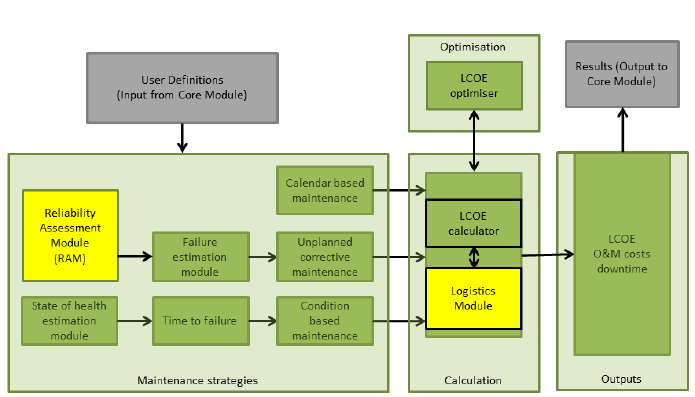
Fig. 7.72 O&M module functional structure

Once all of the required classes are initialised, the optimisation loop (“Calculation” block) runs and sequentially calls several logistic functions to execute the O&M cost calculation. The loop will run until the minimum LCOE is achieved. The optimisation process is rather complex and is described in (DTOcean, 2015i) in detail.

Module structure

The software structure of the O&M module is developed in an object oriented form and is depicted in the Fig. 7.73 below.

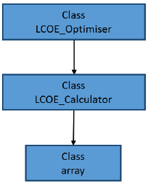
Fig. 7.73 O&M module structure

Class LCOE_Optimiser: This class is reserved for the implementation of the optimisation strategy of the O&M module. The function “executeOptim()” contains the optimisation code which will be called by “ call ” func- tion of LCOE_Optimiser. The class LCOE_Optimiser contains an instance of class LCOE_Calculator. The outputs of the O&M module are collected in a Python dictionary labelled “outputWP6”.

Class LCOE_Calculator: This class is the realisation of the LCOE calculation. The function “executeCalc()” will contain the calculation code of LCOE which will be called by the “ call ” function of LCOE_Calculator. The class LCOE_Calculator contains an instance of array class.

Class array (arrayClass.py): the class array contains all of the information concerning the failure rates, Poisson events etc. in the form of a Python dictionary.

Included Libraries and DTOcean packages

To calculate of optimal LCOE relating to the O&M activities, the dtocean-operation-maintenance package (as the Python package name for the O&M module) requires the estimation of the logistic efforts which will be carried out in the dtocean-logistics package. For the estimation of the down time of the devices the failure rates of components are required which will be calculated in dtocean-reliability package.

Additionally, dtocean-operation-maintenance requires a number of external Python libraries for its operation. These include:

pandas

numpy

SciPy

7.5.3. Functional Specification¶

7.5.3.1. Inputs¶

To execute the module, the following information is required:

the array layout with the number of devices, the exact absolute positions of the devices and the total energy yield for each device;

the internal grid layout (star, loop, etc.), the type of the substation (simple connector or transformer, switch gear, etc.) and the export cable specification

the information about the implementation of the reaction/station-keeping subsystem

the information about the availability, cost and access time of any logistic items, i.e. vessels, jack-up barges, cable laying vessels, etc., but also including specialised equipment (ROVs) and expert personnel (special technicians, divers, etc.)

the annual failure rates for all components for the OEC of interest

To run the O&M module, the user needs to define the information describing all relevant maintenance operations which can be applied to the devices in the array. Possible maintenance operations include simple inspections with maintenance technicians using a small crew transfer vessel (CTV) up to the replacement of a nacelle of a tidal turbine using a jack-up barge and a 100t crane. The required parameters are listed in the table below:

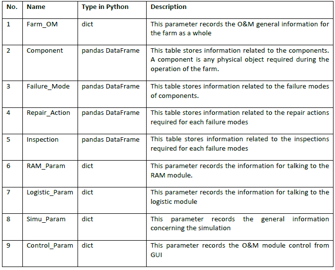
Fig. 7.74 Required user inputs for the Operations and Maintenance module

The full list of the O&M module input parameters with their individual key values is in the following tables. To help define this data, a respective input mask as a template file (Excel format) will be provided on the following pages. This template will allow the user to collect all the required information as mentioned above.

The following table contains the description of the parameters which are common for all components in the array.

The following tables contain the description of the parameters for definition of the electrical components in the array’s balance of plant. There are four parameter categories to be considered:

Category 1: “Component”

Category 2: “FailureModes”

Category 3: “RepairActions”

Category 4: “Inspections”

Notes:

allowed values are “Substation”, “Export Cable”, “Subhub”
Definition of FM IDs

CAPEX costs for condition monitoring hardware: it is assumed that the hardware is not installed in the component/device during production. If the device is purchased with an already installed condition monitoring hardware, set value(s) to “0”;
allowed values for component type
- Hydrodynamic
- Pto
- Control
- Support structure
- Mooring line
- Foundation
- Dynamic cable
- Array elec sub-System

7.5.4. Execution¶

Class inputOM: The interface of the dtocean-operation-maintenance package is implemented as a Python class. The int function of this class takes the defined interface parameters and saves them in internal class parameters. The initialisation of the class is as follows:

def __init__(self,
             Farm_OM,
             Component,
             Failure_Mode,
             Repair_Action,
             Inspection,
             RAM_Param,
             Logistic_Param,
             Simu_Param,
             Control_Param):
   self.__Farm_OM = Farm_OM
   self.__Component = Component
   self.__Failure_Mode = Failure_Mode
   self.__Repair_Action = Repair_Action
   self.__Inspection = Inspection
   self.__RAM_Param = RAM_Param
   self.__Logistic_Param = Logistic_Param
   self.__Simu_Param = Simu_Param
   self.__Control_Param = Control_Param

To run the dtocean-operation-maintenance package the user should make two different instances:

1: An instance of class inputOM:

inputOMPtr = inputOM(Farm_OM,
                     Component,
                     Failure_Mode,
                     Repair_Action,
                     Inspection,
                     RAM_Param,
                     Logistic_Param,
                     Simu_Param,
                     Control_Param)

2: An instance of class LCOE_Optimiser(inputOMPtr): This class contains an instance of class inputOM in order to read the model parameters via this pointer.

ptrOptim = LCOE_Optimiser(inputOMPtr)

For reading the model parameters different getter functions are defined in class inputOM, for instance:

def get_Farm_OM(self):
   return self.__Farm_OM

7.5.4.1. Outputs¶

The execution of the dtocean-operation-maintenance package model is carried out by the following command:

outputOfWP6 = ptrOptim()

outputOfWP6 is the result of the calculations in the O&M module and is a dictionary with the keys defined in Fig. 7.75. The grey shaded variables are combined in the “oputputWP6” structure.

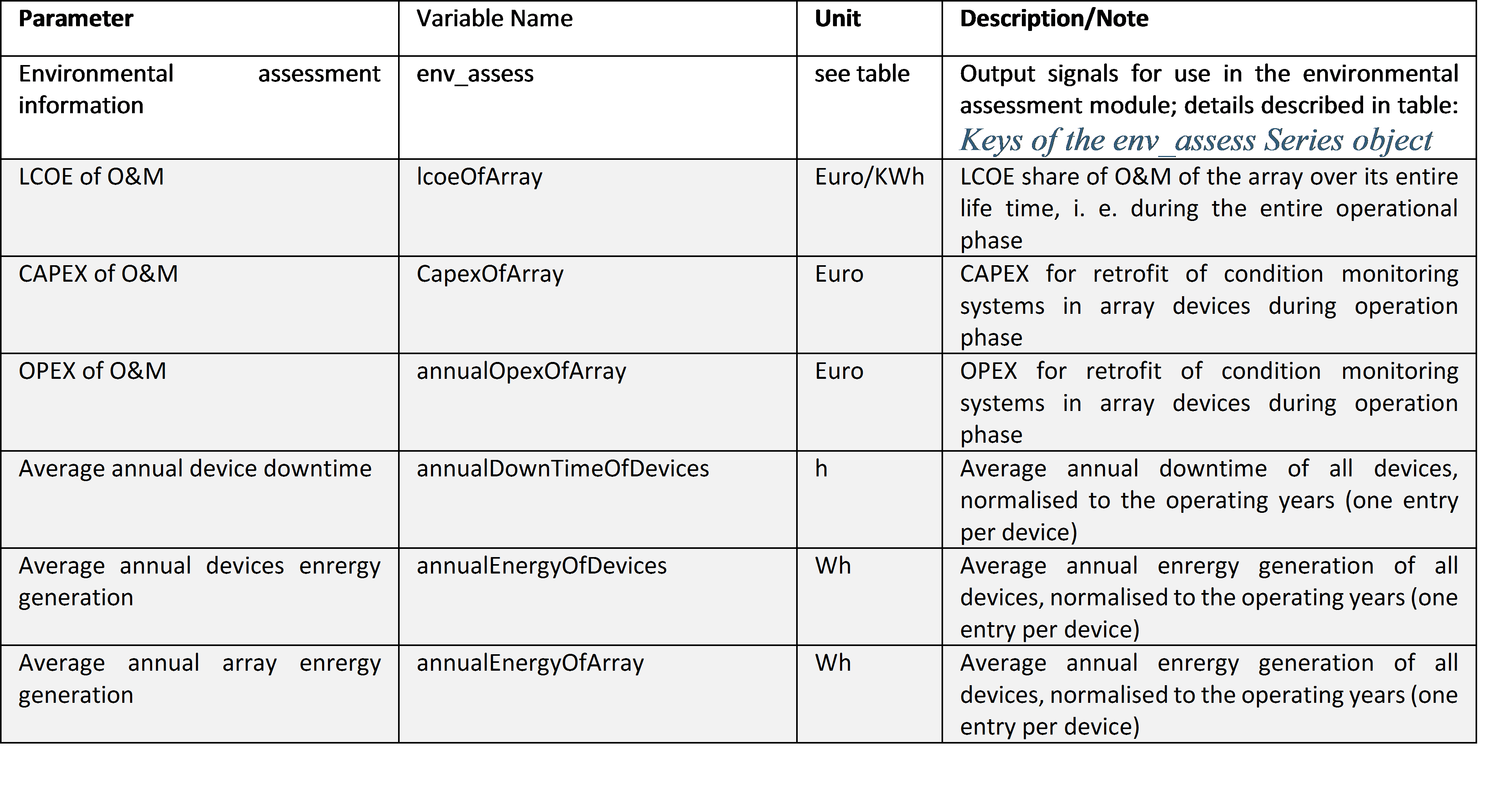
Fig. 7.75 Dictionary keys for the output of the ptrOptim class

Interpretation of env_assess

The env_assess key is formatted as a pandas Series object. Each index (int value) indicates a repair action or an inspection and contains a dictionary with keys seen in Fig. 7.76. The number of indexes in env_assess will match the necessary actions (inspections or repair actions) during the O&M module calculations.

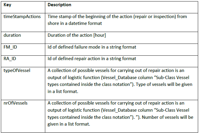
Fig. 7.76 Keys of the env_assess Series object

Interpretation of “outputWP6”

The table below gives some examples for values resulting from a test run with two devices defined in an array.